Predicting the Probability of Default

1. Statistical Models of Default

If you apply for a credit card or a bank loan, you will probably be asked to complete a ques­tionnaire that provides details about your job, home, and financial health. This information is then used to calculate an overall credit score.^[1] If you do not make the grade on the score, you are likely to be refused credit or subjected to a more detailed analysis. In a similar way, mechanical credit scoring systems are used by banks to assess the risk of their corporate loans and by firms when they extend credit to customers.

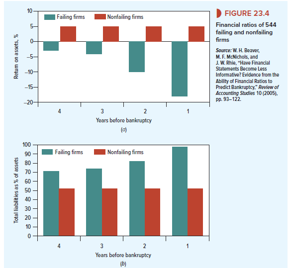
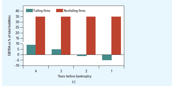
Suppose that you are given the task of developing a system that will help to decide which businesses are poor credits. You start by comparing the financial statements of companies that went bankrupt over a 40-year period with those of surviving firms. Figure 23.4 shows what you find. Panel (a) illustrates that, as early as four years before they went bankrupt, failing firms were earning a much lower return on assets (ROA) than firms that survived. Panel (b) shows that, on average, they also had a high ratio of liabilities to assets, and Panel (c) shows that EBITDA (earnings before interest, taxes, and depreciation) was low relative to the firms’ total liabilities. In each case, these indicators of the firms’ financial health steadily deteriorated as bankruptcy approached.

Rather than focusing on individual ratios, it makes sense to combine the ratios into a single score that can separate the creditworthy sheep from the impecunious goats. That means esti­mating an equation that relates the risk of bankruptcy to a set of financial variables. Most statistical bankruptcy models focus on a relatively small set of accounting ratios. There is gen­eral agreement that the probability of bankruptcy is higher for firms that have low and declin­ing profitability, high debt ratios and low interest coverage, and decreasing cash reserves and working capital.

For small businesses, there may be little alternative to the use of accounting data, but for large, publicly traded firms, it is also possible to take advantage of the information in security prices. Low and volatile stock returns, a low market-to-book ratio, and a low stock price all seem to provide additional information on impending bankruptcy.

Before we leave the topic of these statistical models, we should issue a health warning. When you construct a risk index, it is tempting to experiment with many different combinations of variables until you find the equation that would have worked best in the past. Unfortunately, if you “mine” the data in this way, you are likely to find that the system works less well in the future than it did previously. If you are misled by the past successes into placing too much faith in your model, you could be worse off than if you had pretended that you could not tell one would-be borrower from another and extended credit to all of them. Does this mean that firms should not use credit scoring systems? Not a bit. It merely implies that it is not sufficient to have a good system; you also need to know how much to rely on it.

2. Structural Models of Default

Bankruptcy prediction models use a variety of techniques to estimate the relationship between the occurrence of bankruptcy and the set of financial variables. One of the earliest models that is still widely used is the Z-score model developed by Edward Altman. This used the tech­nique of multiple discriminant analysis to come up with a credit score.^[3] Others have used hazard or probit models. In each case, the user picks a number of variables that he or she suspects might indicate approaching financial distress and then uses a statistical technique to find the combination of these variables that best predicts which firms will become bankrupt.

A different approach is to develop a structural model that builds on the insight that stock­holders will exercise their option to default if the market value of the assets falls below the payments that must be made on the debt. The best known of these models is the Merton model, named after Robert Merton who first developed it,^[4] or Moody’s KMV model, named after the firm that produced a commercial version. We will illustrate with a simple example.

Imagine a company, call it Upsilon, whose assets have a current market value of $100. Its debt has a face value of $60, and the debt matures in one year. The return on the assets has a standard deviation of 30%, so the asset value when the debt matures could be more or less than $60. We assume that the risk-free rate of interest is 5%. Then, if the debt was risk-free, it would be worth 60/1.05 = $57.14. But Upsilon’s debt is risky: If the assets are worth less than $60, the shareholders will exercise their option to default and hand over the assets to the debtholders. The Black-Scholes model tells us that the value of this put option is $0.27. Therefore, the value of the debt is:

Value of debt = value of risk-free debt – value of default put = 57.14 – 0.27 = $56.87

The value of the equity is:

Value of equity = Value of assets – value of debt – 100 – 56.87 = 43.13

To estimate the probability of default, we need to calculate the probability that the put option will be exercised. Figure 23.5 shows the distribution of possible asset values at the end of the year, assuming that investors are risk-neutral and happy to earn the risk-free interest rate on their holdings. The shaded area in the figure shows the probability in a risk-neutral world that the value of the assets at the end of the year will be less than $60 and Upsilon will default. If you look back at the Black-Scholes formula in Section 21-4, you will see the expression N(d₂). The probability that the option will be exercised is equal to 1 – N(d₂). In the case of Upsilon,

Risk-neutral probability of default = 1 – N(d₂) = .043, or 4.3%

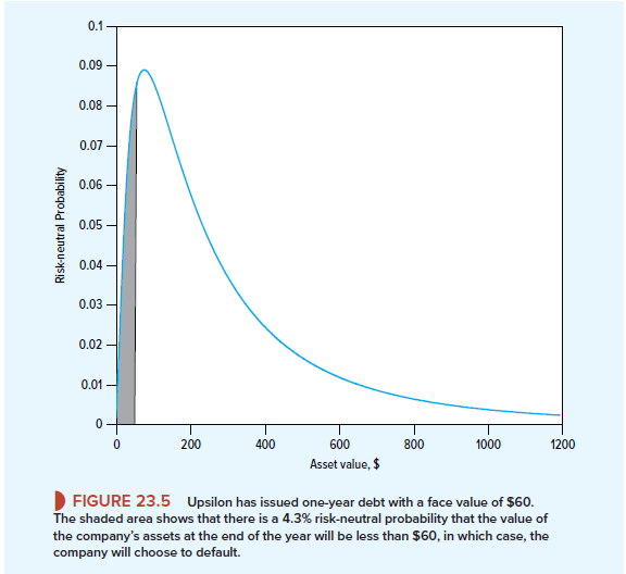
There is a 4.3% chance that Upsilon will default.

The Merton model of default has obvious attractions. It has a theoretical base. So the relevant variables are pretty well known, and you do not need to go prospecting among past data to find variables that may be indications of impending default. But when you apply the model in practice, you inevitably encounter complications. For example, unless you can observe the value of the company’s debts, you can’t observe the value of its assets or measure their volatility.²⁰ Also, companies may have several debt issues, each with a different maturity. You could use an average time to maturity, but, if you are concerned with the probability of default in the short run, you may wish to place more weight on debt that will shortly need to be repaid.

Source:  Brealey Richard A., Myers Stewart C., Allen Franklin (2020), Principles of Corporate Finance, McGraw-Hill Education; 13th edition.