The fact that a project has a positive NPV does not mean that you should go ahead today. It may be better to wait and see how the market develops.
Suppose that you are contemplating a now-or-never opportunity to build a malted herring factory. In this case, you have an about-to-expire call option on the present value of the factory’s future cash flows. If the present value exceeds the cost of the factory, the call option’s payoff is the project’s NPV. But if NPV is negative, the call option’s payoff is zero because, in that case, the firm will not make the investment.
Now suppose that you can delay construction of the plant. You still have the call option, but you face a trade-off. If the outlook is highly uncertain, it is tempting to wait and see whether the malted herring market takes off or decays. On the other hand, if the project is truly profitable, the sooner you can capture the project’s cash flows, the better. If the cash flows are high enough, you will want to exercise your option right away.
The cash flows from an investment project play the same role as dividend payments on a stock. When a stock pays no dividends, an American call is always worth more alive than dead and should never be exercised early. But payment of a dividend before the option matures reduces the ex-dividend price and the possible payoffs to the call option at maturity. Think of the extreme case: If a company pays out all its assets in one bumper dividend, the stock price must be zero and the call worthless. Therefore, any in-the-money call would be exercised just before this liquidating dividend.
Dividends do not always prompt early exercise, but if they are sufficiently large, call option holders capture them by exercising just before the ex-dividend date. We see managers acting in the same way: When a project’s forecasted cash flows are sufficiently large, managers capture the cash flows by investing right away. But when forecasted cash flows are small, managers are inclined to hold on to their call rather than to invest, even when project NPV is positive.[1] This explains why managers are sometimes reluctant to commit to positive-NPV projects. This caution is rational as long as the option to wait is open and sufficiently valuable.
1. Valuing the Malted Herring Option
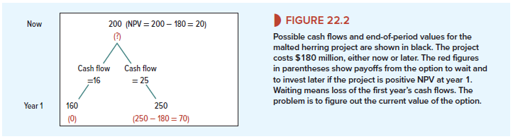
Figure 22.2 shows the possible cash flows and end-of-year values for the malted herring project. If you commit and invest $180 million, you have a project worth $200 million. If demand turns out to be low in year 1, the cash flow is only $16 million and the value of the project falls to $160 million. But if demand is high in year 1, the cash flow is $25 million and value rises to $250 million. Although the project lasts indefinitely, we assume that investment cannot be postponed beyond the end of the first year, and therefore we show only the cash flows for the first year and the possible values at the end of the year. Notice that if you undertake the investment right away, you capture the first year’s cash flow ($16 million or $25 million); if you delay, you miss out on this cash flow, but you will have more information on how the project is likely to work out.
We can use the binomial method to value this option. The first step is to pretend that investors are risk neutral and to calculate the probabilities of high and low demand in this risk-neutral world. If demand is high in the first year, the malted herring plant has a cash flow of $25 million and a year-end value of $250 million. The total return is (25 + 250)/200 – 1 = .375, or 37.5%. If demand is low, the plant has a cash flow of $16 million and a year-end value of $160 million. Total return is (16 + 160)/200 – 1 = -.12, or -12%. In a risk-neutral world, the expected return would be equal to the interest rate, which we assume is 5%:
![]()
Therefore, the risk-neutral probability of high demand is 34.3%. This is the probability that would generate the risk-free return of 5%.
We want to value a call option on the malted herring project with an exercise price of $180 million. We begin as usual at the end and work backward. The bottom row of Figure 22.2 shows the possible values of this option at the end of the year. If project value is $160 million, the option to invest is worthless. At the other extreme, if project value is $250 million, option value is $250 – 180 – $70 million.
To calculate the value of the option today, we work out the expected payoffs in a risk- neutral world and discount at the interest rate of 5%. Thus, the value of your option to invest in the malted herring plant is
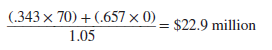
But here is where we need to recognize the opportunity to exercise the option immediately. The option is worth $22.9 million if you keep it open, and it is worth the project’s immediate NPV (200 – 180 _ $20 million) if exercised now. Therefore, we decide to wait and then to invest next year only if demand turns out high.
We have, of course, simplified the malted herring calculations. You won’t find many actual investment-timing problems that fit into a one-step binomial tree. But the example delivers an important practical point: A positive NPV is not a sufficient reason for investing. It may be better to wait and see.
2. Optimal Timing for Real Estate Development
Sometimes it pays to wait for a long time, even for projects with large positive NPVs. Suppose you own a plot of vacant land in the suburbs.[2] The land can be used for a hotel or an office building, but not for both. A hotel could be later converted to an office building, or an office building to a hotel, but only at significant cost. You are therefore reluctant to invest, even if both investments have positive NPVs.
In this case, you have two options to invest, but only one can be exercised. You therefore learn two things by waiting. First, you learn about the general level of cash flows from development—for example, by observing changes in the value of developed properties near your land. Second, you can update your estimates of the relative size of the hotel’s future cash flows versus the office building’s.
Figure 22.3 shows the conditions in which you would finally commit to build either the hotel or the office building. The horizontal axis shows the current cash flows that a hotel would generate. The vertical axis shows current cash flows for an office building. For simplicity, we assume that each investment would have an NPV of exactly zero at a current cash flow of 100. Thus, if you were forced to invest today, you would choose the building with the higher cash flow, assuming the cash flow is greater than 100. (What if you were forced to decide today and each building could generate the same cash flow, say, 150? You would flip a coin.)
If the two buildings’ cash flows plot in the colored area at the lower right of Figure 22.3, you build the hotel. To fall in this area, the hotel’s cash flows have to beat two hurdles. First, they must exceed a minimum level of about 240. Second, they must exceed the office building’s cash flows by a sufficient amount. If the situation is reversed, with office building cash flows above the minimum level of 240, and also sufficiently above the hotel’s, then you build the office building. In this case, the cash flows plot in the colored area at the top left of the figure.
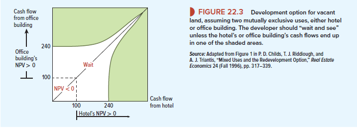
Notice how the “wait and see” region extends upward along the 45-degree line in Figure 22.3. When the cash flows from the hotel and office building are nearly the same, you become very cautious before choosing one over the other.
You may be surprised at how high cash flows have to be in Figure 22.3 to justify investment. There are three reasons. First, building the office building means not building the hotel, and vice versa. Second, the calculations underlying Figure 22.3 assumed cash flows that were small, but growing; therefore, the costs of waiting to invest were small. Third, the calculations did not consider the threat that someone might build a competing hotel or office building right next door. In that case, the “relax and wait” area of Figure 22.3 would shrink dramatically.
Pretty nice post. I simply stumbled upon your weblog and wanted to say that I’ve really enjoyed browsing your blog posts. In any case I’ll be subscribing for your feed and I’m hoping you write once more soon!