Although the democratic process of giving equal weight to each study has some appeal, the reality is that some studies provide better effect size estimates than others, and therefore should be given more weight than others in aggregating results across studies. In this section, I describe the logic of using different weights based on the precision of the effect size estimates.
The idea of the precision of an effect size estimate is related to the standard errors that you computed when calculating effect sizes (see Chapters 5-7). Consider two hypothetical studies: the first study relied on a sample of 10 individuals, finding a correlation between X and Y of .20 (or a Fisher’s transformation, Zr, of . 203); and the second study relied on a sample of 10,000 individuals, finding a correlation between X and Y of .30 (Zr = .310). Before you take a simple average of these two studies to find the typical correlation between X and Y,1 it is important to consider the precision of these two estimates of effect size. The first study consisted of only 10 participants, and from the equation for the standard error of Zr (SE = 1/V(N – 3); see Chapter 5), I find that the expectable deviation in Zr from studies of this size is .378. The second study consisted of many more participants (10,000), so the parallel standard error is 0.010. In other words, a small sample gives us a point estimate of effect size (i.e., the best estimate of the population effect size that can be made from that sample), but it is possible that the actual effect size is much higher or lower than what was found. In contrast, a study with a large sample size is likely to be much more precise in estimating the population effect size. More formally, the standard error of an effect size, which is inversely related to sample size,2 quantifies the amount of imprecision in a particular study’s estimate of the population effect size.
Figure 8.1 further illustrates this concept of precision of effect sizes. In this figure, I have represented five studies of varying sample size, and therefore varying precision in their estimates of the population effect sizes. In this figure, I am in the fortunate—if unrealistic—position of knowing the true population effect size, represented as a vertical line in the middle of the figure. Study 1 yielded a point estimate of the effect size (represented as the circle to the right of this study) that was considerably lower than the true effect size, but this study also had a large standard error, and the resulting confidence interval of that study was large (represented as the horizontal arrow around this effect size). If I only had this study to consider, then my best estimate of the population would be too low, and the range of potential effect sizes (i.e., the horizontal range of the confidence interval arrow) would be very large. Note that the confidence interval of this study does include the true population effect size, but this study by itself is of little value in determining where this unknown value lies.
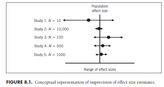
The second study of Figure 8.1 includes a large sample. You can see that the point estimate of the effect size (i.e., the circle to the right of this study) is very close to the true population effect size. You also see that the confidence interval of this study is very narrow; this study has a small standard error and therefore high precision in estimating the population effect size. Clearly, the results of this study offer a great deal of information in determining where the true population effect size lies, and I therefore would want to give more weight to these results than to those from Study 1 when trying to determine this population effect size.
The remaining three studies in Figure 8.1 contain sample sizes between those of Studies 1 and 2. Two observations should be noted regarding these studies. First, although none of these studies perfectly estimates the population effect size (i.e., none of the circles fall perfectly on the vertical line), the larger studies tend to come closer. Second, and related, the confidence intervals all3 contain the true population effect size.
The crucial difference between the hypothetical situation depicted in Figure 8.1 and reality is that you do not know the true population effect size when you are conducting a meta-analysis. In fact, one of the primary purposes of conducting a meta-analysis is to obtain a best estimate of this population effect size. In other words, you want to decide where to draw the vertical line in Figure 8.1. As I hope is clear at this point, it would make sense to draw this line so that it is closer to the effect size estimates from studies with narrow confidence intervals (i.e., small standard errors), and give less emphasis to ensuring that the line is close to those from studies with wide confidence intervals (i.e., large standard errors). In other words, you want to give more weight to some studies (those with small standard errors) than to others (those with large standard errors).
How do you quantify this differential weighting? Although the choices are virtually limitless,4 the statistically defensible choice is to weight effect sizes by the inverse of their variances in point estimates (i.e., standard errors squared). In other words, you should determine the weight of a particular study i (wj) from the standard error of the effect size estimate from that study (SEj) using the following equation:
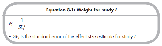
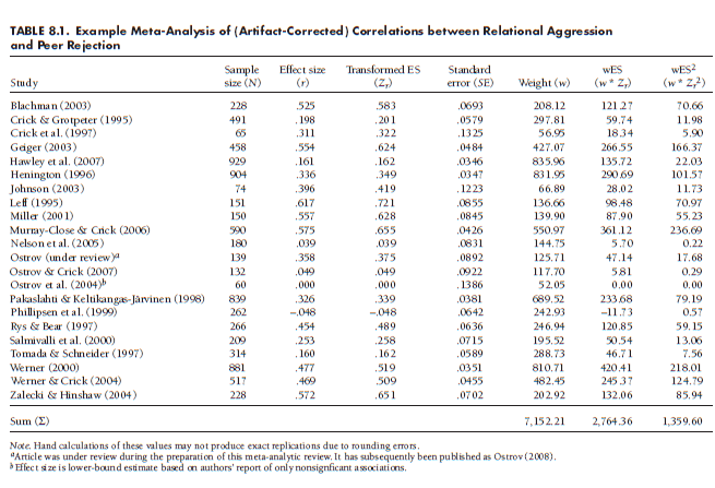
In all analyses I describe in this chapter, you will use this weight. I suggest that you make a variable in your meta-analytic database representing this weight for each study in your meta-analysis. In the running example of this chapter, shown in Table 8.1, I consider 22 studies providing correlations between relational aggression and peer rejection. In addition to listing the study, I have columns showing the sample size, corrected effect sizes in original r and transformed Zr metrics, and the standard errors (SEzr) of these estimates. Note that these effect sizes have been corrected for two artifacts (see Chapter 6)—unreliability and artificial dichotomization (when relevant)—so the standard errors are also adjusted and not directly computable from sample size (for details, see Chapter 6). This table also shows the weight (w) for each study, computed from the standard errors using Equation 8.1.
Source: Card Noel A. (2015), Applied Meta-Analysis for Social Science Research, The Guilford Press; Annotated edition.
25 Aug 2021
25 Aug 2021
24 Aug 2021
25 Aug 2021
24 Aug 2021
24 Aug 2021