Design Weights of Survey Data in Stata

The previous section took weight definitions for granted, and indeed many data users begin with a completed survey in which weights have already been calculated by someone else. This and the following sections present examples showing how such calculations are done.

Survey researchers apply probability weights to adjust for biases in their sampling methods. The biases could arise from intentional features of the sampling design, or from accidental properties of the data-collection process. Either way, initial sampling yields data not well representing the population of interest. Probability weighting attempts to compensate for departures from simple random sampling, and give us a more realistic picture of sampling variability and population characteristics.

For the Granite State Poll, interviewers call a random sample of New Hampshire household telephone numbers. In theory, these random phone numbers could yield a representative sample of households. For voting research and many other purposes, however, pollsters want to generalize not about the population of households, but about the population of adults (or voters) living in those households. Some households contain only one adult, whereas others have more. Among respondents to the June 2011 poll, about 29% said that they lived in a one-adult household. Responses in this example are limited to one, two, or three or more adults, as a practical compromise for weighting purposes. Only 503 of the original 516 respondents gave an answer regarding the number of adults; we will return to the other 13 later.

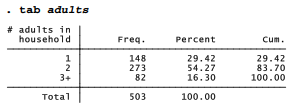
Although 29% of our sample lived in one-adult households, it would be a mistake to guess that a similar percentage of New Hampshire adults do so. To select a resident randomly, once a household has been called, the telephone interviewers ask to speak to the adult in the household who had the most recent birthday, or would call back later if that individual was not present. People from households with one adult therefore were at least three times more likely to enter our sample, compared with those from households with three or more. The table above suggest that our phone calls reached households with at least (1*148)+(2*273)+(3×82) = 940 adults. Among this sample of pseudo-people, those living in one-adult households make up only 148/940 or 16%, much less than the 29% in our table.

Survey weights provide a way to adjust for such known sampling biases, and achieve more realistic results. In this example that could matter not only for describing household size, but for other things such as voting behavior that might be correlated with household size. Single-adult households probably include a larger proportion of elderly people living alone. Two-adult households will include many young families. Multi-adult households will often be older families with adult children, or else young adults with roommates.

Probability weights are proportional to the inverse of the probability of selection. For our example, the conditional probability of selecting a particular person from a one-adult household (given that we phoned there) equals one. The probability of selecting a person from a two- person household equals 1/2, and from a three-person household 1/3. If we used the inverse of these probabilities, 1, 2 and 3, as weights then our sample would contain 940 pseudo-people — giving us the correct proportions, but leading to incorrect totals and other confusion. To maintain the true sample size, we can multiply these inverse probabilities by the ratio of real people to pseudo-people, 503/940. This step creates a new variable named adultwt, which contains the probability weights to adjust for a known sampling bias, while preserving the original sample size. The weights are .535 (one-adult household), 1.070 (two adults) or 1.605 (three or more); missing values get a neutral weight of 1. The ratio of these weights remains 1:2:3.

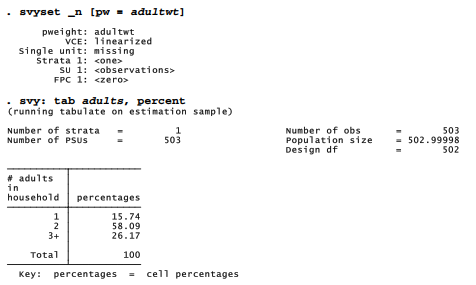
The weighted proportions (such as 16% from one-person households, instead of 29% as in the raw data) give a more realistic picture.

Source: Hamilton Lawrence C. (2012), Statistics with STATA: Version 12, Cengage Learning; 8th edition.