Smoothing by using Stata

Many time series exhibit high-frequency variations that make it difficult to discern underlying patterns. Smoothing such series breaks the data into two parts, one that varies gradually, and a second “rough” part containing the leftover rapid changes:

data = smooth + rough

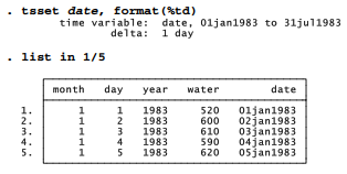
To illustrate smoothing methods, we examine data on daily water consumption for the town of Milford, New Hampshire over seven months from January through July 1983 (MILwater.dta; source Hamilton 1985). Milford’s usual patterns of water use were interrupted by alarming news midway through this period.

Before further analysis, we need to convert the month, day and year information into a single numerical index of time. Stata’s mdy( ) function does this, creating an elapsed-date variable (named date here) indicating the number of days since January 1, 1960.

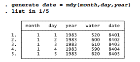
The January 1, 1960 reference date is arbitrary but fixed. We can provide more understandable formatting for date, and also set up our data for later analyses, by using the tsset (time series set) command to identify date as the time index variable and to specify the %td (daily) display option for this variable.

Dates in the new date format, such as “05jan1983”, are more readable than the underlying numeric values such as “8405” (days since January 1, 1960). If desired, we could use %td formatting to produce other formats, such as “05 Jan 1983” or “01/05/83”. Stata offers a number of variable-definition, display-format and dataset-format features that are important with time series. Many of these involve ways to input, convert and display dates. Full descriptions of date functions are found in the Data Management Reference Manual and the User’s Guide, or they can be explored within Stata by typing help dates.

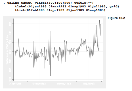
Figure 12.1 uses twoway line to draw a simple time plot of water against date. The graph shows a pattern of day-to-day variation, as well as an upward trend in water use when summer arrives. Values for our date-format variable are labeled automatically (01jan1983, etc.) on the x (or t) axis, but Stata’s default choices here lead to crowded, unsatisfactory results.

A better way to draw time plots when the x axis is a date variable is to use the special time series command tsline. This command allows us to describe the x axis in terms of dates, without having to reference the numerical elapsed dates underneath. For example, we could draw a time plot similar to Figure 12.1 but with a less crowded time axis, as seen in Figure 12.2 on the next page. Note that the tsline command does not accept an x variable, only one or more y variables. With tsset data, the time dimension has already been defined. Options tlabel( ) and ttick( ) work in a tsline plot just as xlabel( ) and xtick( ) would in any other twoway plot, except that they understand date notations such as 01jan1983. In Figure 12.2 we have also suppressed the x-axis (time or t-axis) title with the option ttitle(“”), because the word “Date” there seems superfluous below an axis labeled 01jan1983, 01mar1983 and so forth.

Visual inspection plays a key role in time series analysis. Smoothing often helps us to see underlying patterns beneath jagged series. The simplest smoothing method is to calculate a moving average at each data point based on present, earlier and later values ofy. For example, a “moving average of span 3” refers to the mean of y_t-1 , y_t and y_;+1 . We could use Stata’s explicit subscripting to generate such a variable:

. generate water3a = (water[_n-1] + water[_n] + water[_n+1])/3

A better way involves the ma (moving average) function of egen :

. egen water3b = ma(water), nomiss t(3)

The nomiss option in this egen command requests shorter, uncentered moving averages in the tails; otherwise, the first and last values of water3 would be missing. The t(3) option calls for moving averages of span 3. Any odd-number span of 3 or more could be used.

For time series (tsset) data, powerful smoothing tools are available through the tssmooth commands. All but tssmooth nl can handle missing values.

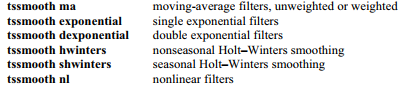
moving-average filters, unweighted or weighted single exponential filters double exponential filters nonseasonal Holt-Winters smoothing seasonal Holt-Winters smoothing nonlinear filters

tssmooth ma, for example, can calculate moving averages of span 3, identical to those from our previous egen command:

Type help tssmooth ma, help tssmooth exponential, etc. for the syntax of each command.

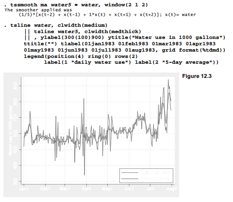
Figure 12.3 graphs a 5-day moving average of Milford water use (waterS), together with the raw data (water). The tsline command overlays a time plot of smoothed water5 values onto a plot of raw water values (thinner line). 7-axis labels mark the dates, as they did in Figure 12.2. In Figure 12.3, however, we specify a simpler date display format giving just the month and day, format(%tdmd). The shorter format leaves room to label the beginning of each month in this graph, as opposed to every other month as previously done in Figure 12.2.

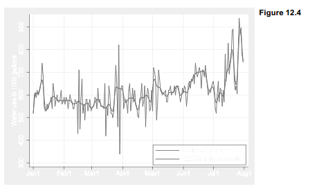
Moving averages share a drawback of other mean-based statistics: they have little resistance to outliers. Because outliers form prominent spikes in the water time series, we might try a more resistant smoothing method. The tssmooth nl command performs outlier-resistant nonlinear smoothing, employing methods and terminology described in Velleman and Hoaglin (1981) and Velleman (1982). For example,

. tssmooth nl water5r = water, smoother(5)

creates a new variable named water5r, holding the values of water after smoothing by running medians of span 5. Compound smoothers using running medians of different spans, in combination with Hanning (%, % and % -weighted moving averages of span 3) and other techniques, can be specified in Velleman’s original notation. One compound smoother that seems particularly useful with data that change rapidly is called “4253h, twice.” Applying this to water, we calculate smoothed variable water4r.

. tssmooth nl water4r = water, smoother(4253h,twice)

Figure 12.4 graphs these new smoothed values, water4r. Compare Figure 12.4 with 12.3 to see how 4253h, twice smoothing performs relative to a span-5 moving average. Although both smoothers have similar spans, 4253h, twice does more to reduce the jagged variations.

Sometimes our goal in smoothing is to look for patterns in smoothed plots. With these particular data, however, the rough or residuals after smoothing actually hold more interest. We can calculate the rough as the difference between data and smooth, and then graph these residuals in their own time plot, as done in Figure 12.5.

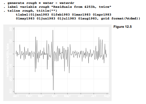
The wildest fluctuations in Figure 12.5 occur around March 27-29. Water use abruptly dropped, rose again, and then dropped lower and bounced even higher before settling towards more usual levels. On these days, local newspapers carried stories that hazardous chemical wastes had been discovered in one of the wells that supplied the town’s water. Initial reports alarmed people, and consumption dropped precipitously. Over the next few days, water use vacillated between high and low peaks, in response to new developments or in compensation for delayed use. Things calmed down after the questionable well was taken offline.

Source: Hamilton Lawrence C. (2012), Statistics with STATA: Version 12, Cengage Learning; 8th edition.