Autoregressive integrated moving average (ARIMA) models can be estimated through the arima command. This command encompasses autoregressive (AR), moving average (MA), or ARIMA models. It also can estimate structural models that include one or more predictor variables and ARIMA disturbances. These are termed ARMAX models, for autoregressive moving average with exogenous variables. The general form of such ARMAX models, in matrix notation, is
![]()
where yt is the vector of dependent-variable values at time t, xt is a matrix of exogenous predictor-variable values (usually including a constant), and p, is a vector of “everything else” disturbances. Those disturbances can be autoregressive or moving-average, of any order. For example, ARMA(1,1) disturbances are
![]()
where pis a first-order autoregressive parameter, Pis a first-order moving average parameter, and et represents random, uncorrelated white-noise (normal i.i.d.) errors. arima fits simple models as a special case of [12.1] and [12.2], with a constant (p0) replacing the structural term xt /i. Therefore, a simple ARMA(1,1) model becomes
![]()
Some sources present an alternative version. In the ARMA(1,1) case, they show yt as a function of the previous y value (yt-1) and the present (e;) and lagged (e;-1) disturbances:
![]()
Because in the simple structural model y, = 0o + pt, equation [12.3] (employed by Stata) is equivalent to [12.4], apart from rescaling the constant a = (1-p)^0 .
Using the arima command, an ARMA(1,1) model can be specified in either of two ways:
. arima y, ar(1) ma(1)
or
. arima y, arima(1,0,1)
The i in arima stands for “integrated,” referring to models that also involve differencing. To fit an ARIMA(2,1,1) model, use
. arima y, arima(2,1,1)
or equivalently,
. arima D.y, ar(1/2) ma(1)
Note that within the arima() option, the number given for autoregressive or moving average terms specifies all lags up to and including that number, so “2” means both lags 1 and 2. When the ar() or ma() options are used, however, the number specifies only that particular lag, so “2” means a lag of 2 only. Either command above specifies a model in which first differences of the dependent variable (yt – yt-1) are a function of first differences one and two lags previous (yt-1 – yt-2 and yt-2 – yt-3), and also of present and previous errors (e, and et-1).
To estimate a structural model in which yt depends on two predictor variables x (present and lagged values, xt and xt-1) and w (present values only, wt), with ARIMA(1,0,3) errors and also multiplicative seasonal ARIMA(1,0,1)12 errors looking back 12 periods (as might be appropriate for monthly data, over a number of years), a suitable command could have the form
. arima y x L.x w, arima(1,0,3) sarima(1,0,1,12)
In econometric notation, this corresponds to an ARIMA(1,0,3)x(1,0,1)12 model.
A time series y is considered stationary if its mean and variance do not change with time, and if the covariance betweeny t andyt+u depends only on the lag u, and not on the particular values of t. ARIMA modeling assumes that our series is stationary, or can be made stationary through appropriate differencing or transformation. We can check this assumption informally by inspecting time plots for trends in level or variance. We have already seen that global temperature, for example, exhibits a clear trend, suggesting that it is not stationary.
Formal statistical tests for “unit roots,” a nonstationary AR(1) process in which p1 = 1 (also known as a random walk), supplement theory and informal inspection. Stata offers three unit root tests: pperron (Phillips-Perron), dfuller (augmented Dickey-Fuller) and dfgls (augmented Dickey- Fuller using GLS). dfgls is the most powerful and informative.
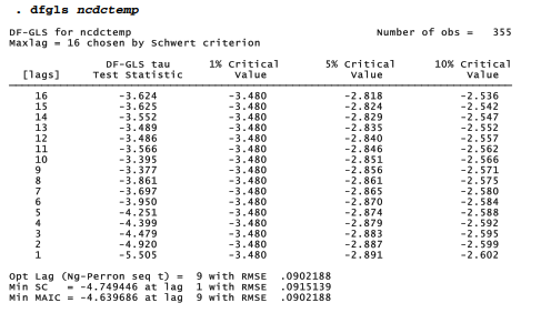
The table below applies dfgls to the National Climate Data Center (NCDC) global temperature anomalies.
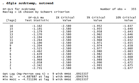
The dfgls output above reports tests of the nonstationary null hypothesis — that the temperature series represents a random walk, or has a unit root — for lags from 1 to 16 months. At the bottom, the output offers three different methods for choosing an appropriate number of lags: Ng-Perron sequential t, minimum Schwarz information criteria, and Ng-Perron modified
Akaike information criteria (MAIC). The MAIC is more recently developed, and Monte Carlo experiments support its advantages over the Schwarz method. Both sequential t and MAIC recommend 9 lags. The DF-GLS statistic for 9 lags is -1.204, greater than the 10% critical value of -1.658, so we should not reject the null hypothesis. These results confirm earlier impressions that the ncdctemp time series is not stationary.
A similar test of the Multivariate ENSO Index, on the other hand, rejects the nonstationary null hypothesis at all lags, even at the 1% level.
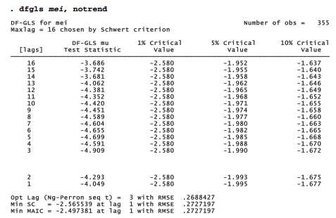
For a stationary series such as mei, correlograms provide guidance about selecting a preliminary ARIMA model:
AR(p) An autoregressive process of order p has autocorrelations that damp out gradually with increasing lag. Partial autocorrelations cut off after lag p.
MA(q) A moving average process of order q has autocorrelations that cut off after lag Partial autocorrelations damp out gradually with increasing lag.
ARMA(p,q) A mixed autoregressive-moving average process has autocorrelations and partial autocorrelations that damp out gradually with increasing lag.
Correlogram spikes at seasonal lags (for example, at 12, 24 or 36 in monthly data) indicate a seasonal pattern. Identification of seasonal models follows similar guidelines, applied to autocorrelations and partial autocorrelations at seasonal lags.
We have seen that autocorrelations for mei damp out gradually with increasing lag (Figure 12.14), while partial autocorrelations cut off after lag 2. These correlogram patterns, together with dfgls test results supporting stationarity, suggest that mei could be modeled as an ARIMA(2,0,0) process.
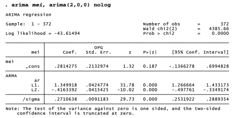
This ARIMA(2,0,0) model represents mei as a function of disturbances (u) from one and two previous months, plus random white-noise errors (e):
![]()
where y, is the value of mei at time t. The output table gives parameter estimates p0 = .28, p1 = 1.35 and p2 = -.42.
After we fit an arima model, these estimates and other results are saved temporarily in Stata’s usual way. For example, to see the model’s AR(1) coefficient and standard error, type
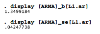
Both the first and second-order autoregressive coefficients in this example are significant and far from zero (t = 31.78 and -10.02, respectively), which gives one indication of model adequacy. We can obtain predicted values, residuals and other case statistics after arima through predict:
. predict meihat
. label variable meihat “predicted MEI”
. predict meires, resid . label variable meires “residual MEI”
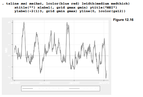
Graphically, predicted values from this model appear almost indistinguishable from the observed temperatures (Figure 12.16). This image highlights how closely ARIMA models can fit strongly autocorrelated series, by predicting a variable from its own previous values, plus the values of previous disturbances. The ARIMA(2,0,0) model explains about 92% of the variance in mei.
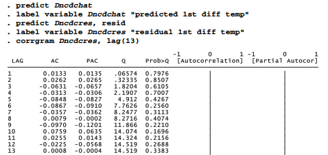
An important test of ARIMA model adequacy is whether the residuals appear to be uncorrelated white noise. corrgram tests the white-noise null hypothesis across different lags.
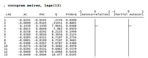
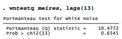
corrgram’s portmanteau Q tests find no significant autocorrelation among residuals out to lag 13, apart from one just below the .05 level at lag 3. We could obtain the same test for any specific lag using a wntestq command, such as
Thus, the ARIMA(2,0,0) model originally proposed after looking at correlogram patterns turns out to fit quite well, with both of its AR terms significant. It leaves residuals that pass tests for white noise.
Our earlier dfgls, notrend test for global temperature anomalies (ncdctemp), unlike the test for Multivariate ENSO Index (mei), found that temperature appears nonstationary because it contains a prominent trend. A default dfgls test that includes a linear trend rejects the nonstationary null hypothesis at all lags.
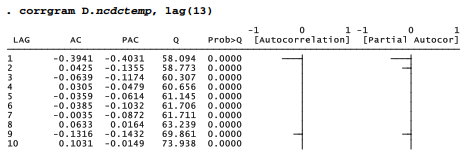
First differencing time series will remove a linear trend. First differences of temperature show a pattern of autocorrelations that cut off after lag 1, and partial autocorrelations that damp out after lag 1.
![]()
These observations suggest that an ARIMA(0,1,1) model might be appropriate for temperatures.
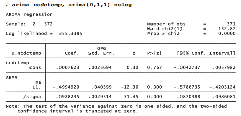
This ARIMA(0,1,1) model describes the first difference or month-to-month change in temperature as a function of present and 1-month lagged random noise:
![]()
where y trepresents ncdctemp at time t. Parameter estimates are p0 = .00076 and d= -.499. The first-order MA term, d, is statistically significant (p ~ 0.000), and the model’s residuals are indistinguishable from white noise.
Although these tests give no reason to discard our ARIMA(0,1,1), the month-to-month changes in global temperature anomaly prove relatively hard to predict. Figure 12.17 employs the difference operator D. in a graph command to show the unimpressive fit between observed and predicted values. This model explains only about 20% of the variance in monthly differences.
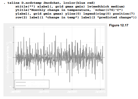
The plot of changes or first differences in Figure 12.17 bears little resemblance to the temperature anomalies themselves, seen in Figure 12.9. The contrast serves to emphasize that modeling first differences answers a different research question. In this example, a key feature of the temperatures record — the upward trend — has been set aside. The next section returns to the undifferenced anomalies and considers how the trend itself could be explained.
Source: Hamilton Lawrence C. (2012), Statistics with STATA: Version 12, Cengage Learning; 8th edition.
I don’t unremarkably comment but I gotta tell regards for the post on this one : D.