Aggregate Planning Using Linear Programming in a Supply Chain

As we discussed earlier, the goal of aggregate planning is to maximize profit while meeting demand. Every company, in its effort to meet customer demand, faces certain constraints, such as the capacity of its facilities or a supplier’s ability to deliver a component. A highly effective tool for a company to use when it tries to maximize profits while being subjected to a series of constraints is linear programming. Linear programming finds the solution that creates the highest profit while satisfying the constraints that the company faces. We now illustrate a lin­ear programming approach to aggregate planning using Red Tomato Tools.

1. Decision Variables

The first step in constructing an aggregate planning model is to identify the set of decision vari­ables whose values are to be determined as part of the aggregate plan. For Red Tomato, the fol­lowing decision variables are defined for the aggregate planning model:

W_t = workforce size for Month t, t = 1, . . . , 6

H_t = number of employees hired at the beginning of Month t, t = 1,         .   . . , 6

L_t = number of employees laid off at the beginning of Month t, t =         1, . .    .  , 6

P_t = number of units produced in Month t, t = 1, . . . , 6 I_t = inventory at the end of Month t, t = 1, . . . , 6

S_t = number of units stocked out/backlogged at the end of Month t, t = 1, . . . , 6

C_t = number of units subcontracted for Month t, t = 1, . . . , 6

O_t = number of overtime hours worked in Month t, t = 1, . . . , 6

The next step in constructing an aggregate planning model is to define the objective function.

2. Objective Function

Denote the demand in Period t by D_t. The values of D_t are as specified by the demand forecast in Table 8-2. The objective function is to minimize the total cost (equivalent to maximizing total profit as all demand is to be satisfied) incurred during the planning horizon. The cost incurred has the following components:

• Regular-time labor cost
• Overtime labor cost
• Cost of hiring and layoffs
• Cost of holding inventory
• Cost of stocking out
• Cost of subcontracting
• Material cost

These costs are evaluated as follows:

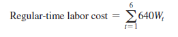
1. Regular-time labor cost. Recall that workers are paid a regular-time wage of $640 ($4/hour X 8 hours/day X 20 days/month) per month. Because W_t is the number of workers in Period t, the regular-time labor cost over the planning horizon is given by

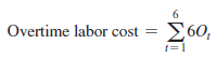
2. Overtime labor cost. As overtime labor cost is $6 per hour (see Table 8-3) and O_t represents the number of overtime hours worked in Period t, the overtime cost over the planning horizon is

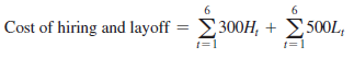
3. Cost of hiring and layoffs. The cost of hiring a worker is $300 and the cost of laying off a worker is $500 (see Table 8-3). H_t and L_t represent the number hired and the number laid off, respectively, in Period Thus, the cost of hiring and layoff is given by

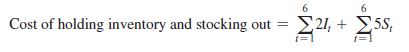
4. Cost of inventory and stockout. The cost of carrying inventory is $2 per unit per month, and the cost of stocking out is $5 per unit per month (see Table 8-3). I_t and S_t represent the units in inventory and the units stocked out, respectively, in Period Thus, the cost of holding inventory and stocking out is

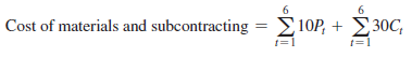
5. Cost of materials and subcontracting. The material cost is $10 per unit and the sub­contracting cost is $30/unit (see Table 8-3). P_t represents the quantity produced and C_t represents the quantity subcontracted in Period t. Thus, the material and subcontracting cost is

The total cost incurred during the planning horizon is the sum of all the aforementioned costs and is given by

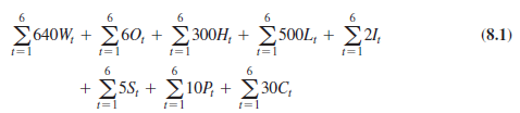
Red Tomato’s objective is to find an aggregate plan that minimizes the total cost (Equation 8.1) incurred during the planning horizon.

The values of the decision variables in the objective function cannot be set arbitrarily. They are subject to a variety of constraints defined by available capacity and operating policies. The next step in setting up the aggregate planning model is to define clearly the constraints linking the decision variables.

3. Constraints

Red Tomato’s vice president must now specify the constraints that the decision variables must not violate. They are as follows:

1. Workforce, hiring, and layoff constraints. The workforce size W_t in Period t is obtained by adding the number hired H_t in Period t to the workforce size W_t-1 in Period t – 1, and subtracting the number laid off L_t in Period t as follows:

Wt = Wt – 1 + Ht – Lt   for    t = 1, . . . , 6                    ( 8.2)

2. Capacity constraints. In each period, the amount produced cannot exceed the avail­able capacity. This set of constraints limits the total production by the total internally available capacity (which is determined based on the available labor hours, regular or overtime). Subcon­tracted production is not included in this constraint because the constraint is limited to produc­tion within the plant. As each worker can produce 40 units per month on regular time (four hours per unit as specified in Table 8-3) and one unit for every four hours of overtime, we have the following:

3. Inventory balance constraints. The third set of constraints balances inventory at the end of each period. Net demand for Period t is obtained as the sum of the current demand D_t and the previous backlog S_{t -1}. This demand is either filled from current production (in-house production P_t or subcontracted production C_t) and previous inventory I_t_ ₁ (in which case some inventory I_t may be left over) or part of it is backlogged S_t. This relationship is captured by the following equation:

It _ 1 + Pt + Ct = Dt + St _ i + It _ St for t = 1, . . . , 6                                        (8.4)

The starting inventory is given by I₀ = 1,000, the ending inventory must be at least 500 units (i.e., I₆ > 500), and initially there are no backlogs (i.e., S₀ = 0).

4. Overtime limit constraints. The fourth set of constraints requires that no employee work more than 10 hours of overtime each month. This requirement limits the total amount of overtime hours available as follows:

O_t < 10W_t for t = 1, . . . , 6                                                            (8.5)

In addition, each variable must be nonnegative and there must be no backlog at the end of Period 6 (i.e., S₆ = 0).

When implementing the model in Microsoft Excel, which we discuss later, it is easiest if all the constraints are written so the right-hand side for each constraint is 0. The overtime limit constraint (Equation 8.5) in this form is written as

O_t _ 10W_t < 0 for t = 1, . . . , 6

Observe that one can easily add constraints that limit the amount purchased from subcontrac­tors each month or the maximum number of employees to be hired or laid off. Any other con­straints limiting backlogs or inventories can also be accommodated. Ideally, the number of employees hired or laid off should be integer variables. Fractional variables may be justified if some employees work for only part of a month. Such a linear program can be solved using the tool Solver in Excel.

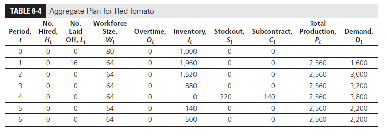
By optimizing the objective function (minimizing cost in Equation 8.1) subject to the listed constraints (Equations 8.2 to 8.5), the vice president obtains the aggregate plan shown in Table 8-4. (Later in the chapter, we discuss how to perform this optimization using Excel with the spread­sheet Chapter8,9-examples.)

For this aggregate plan, we have the following:

Total cost over planning horizon = $422,660

Red Tomato lays off a total of 16 employees at the beginning of January. After that, the company maintains the workforce and production level. It uses the subcontractor during the month of April. Red Tomato carries a backlog only from April to May; in all other months, it plans no stockouts. In fact, it carries inventory in all other periods. We describe this inventory as seasonal inventory because it is carried in anticipation of a future increase in demand.

If the seasonal fluctuation of demand grows, synchronization of supply and demand becomes more difficult, resulting in an increase in either inventory or backlogs as well as an increase in the total cost to the supply chain. This is illustrated in Example 8-1, in which the demand forecast is more variable.

EXAMPLE 8-1 Impact of Higher Demand Variability

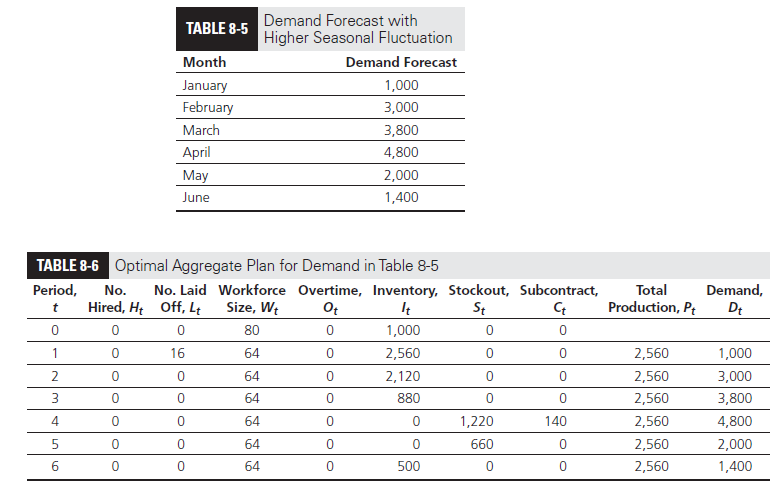
All the data are exactly the same as in our previous discussion of Red Tomato, except for the demand forecast. Assume that the same overall demand (16,000 units) is distributed over the six months in such a way that the seasonal fluctuation of demand is higher, as shown in Table 8-5. Obtain the optimal aggregate plan in this case.

Analysis

In this case, the optimal aggregate plan (using the same costs as those used before) is shown in Table 8-6.

Observe that monthly production remains the same, but both inventories and stockouts (backlogs) go up compared to the aggregate plan in Table 8-4 for the demand profile in Table 8-2. The cost of meeting the new demand profile in Table 8-5 is higher, at $433,080 (compared to $422,660 for the previous demand profile in Table 8-2).

From Example 8-1, we can see that the increase in demand variability at the retailer increases seasonal inventory as well as planned costs.

Using the Red Tomato example, we also see that the optimal trade-off changes as the costs change. This is illustrated in Example 8-2, in which we show that as the costs of hiring and layoff decrease, it is better to vary capacity with demand while having less inventory and fewer backlogs.

EXAMPLE 8-2 Impact of Lower Costs of Hiring and Layoff

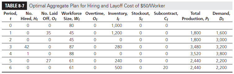
Assume that demand at Red Tomato is as shown in Table 8-2, and all other data are the same except that the costs of hiring and layoff are now $50 each. Evaluate the total cost corresponding to the aggregate plan in Table 8-4. Suggest an optimal aggregate plan for the new cost structure.

Analysis

If the costs of hiring and layoff decrease to $50 each, the cost corresponding to the aggregate plan in Table 8-4 decreases from $422,660 to $412,770. Taking this new cost into account and determining a new optimal aggregate plan yields the plan shown in Table 8-7. Observe that the workforce size fluctuates between a high of 88 and a low of 45, as opposed to being stable at 64 as in Table 8-4.

As expected, the workforce size is varied (because the cost of varying capacity has decreased), whereas inventory and stockouts have decreased compared with the aggregate plan in Table 8-4. The total cost of the aggregate plan in Table 8-7 is $412,770, compared with $422,660 (for the aggregate plan in Table 8-4) if the costs of hiring and layoff are $50 each.

From Example 8-2, observe that increasing volume flexibility (by decreasing the cost of hiring and layoff) not only decreases the total cost but also shifts the optimal balance toward using the volume flexibility while carrying lower inventories and allowing less stockout.

In the next section, we explain how to implement the linear programming methodology for aggregate planning using Microsoft Excel.

Source: Chopra Sunil, Meindl Peter (2014), Supply Chain Management: Strategy, Planning, and Operation, Pearson; 6th edition.