Application 5: Testing Factorial Invariance of Scales from a Measurement Scale (First-Order CFA Model) with AMOS

1. Key Concepts

• Conceptual notion of factorial invariance (i.e., equivalence)
• Analysis of covariance (COVS) versus means and covariance (MaCs) structures
• Evidence of partial measurement invariance
• Hierarchical set of steps involved in testing factorial invariance
• Chi-square-difference versus CFI-difference tests
• Working with multiple groups in Amos
• Manual versus Amos-automated approach to invariance testing

Up to this point, all applications have illustrated analyses based on single samples. In this section, however, we focus on applications involving more than one sample where the central concern is whether or not components of the measurement model and/or the structural model are invariant (i.e., equivalent) across particular groups of interest. Throughout this chapter and others involving multigroup applications, the terms invariance and equivalence are used synonymously (likewise the adjectives, invariant and equivalent); use of either term is merely a matter of preference.

In seeking evidence of multigroup invariance, researchers are typ­ically interested in finding the answer to one of five questions. First, do the items comprising a particular measuring instrument operate equiva­lently across different populations (e.g., gender; age; ability; culture)? In other words, is the measurement model group-invariant? Second, is the factorial structure of a single measurement scale or the dimensional­ity of a theoretical construct equivalent across populations as measured either by items of a single assessment measure or by subscale scores from multiple instruments? Typically, this approach exemplifies a construct validity focus. In such instances, equivalence of both the measurement and structural models are of interest. Third, are certain structural regres­sion paths in a specified path-analytic structure equivalent across pop­ulations? Fourth, is there evidence of differences in the latent means of particular constructs in a model across populations? Finally, does the factorial structure of a measuring instrument replicate across independ­ent samples drawn from the same population? This latter question, of course, addresses the issue of cross-validation. Applications presented in this chapter as well as the next two chapters provide you with spe­cific examples of how each of these questions can be answered using structural equation modeling based on the Amos Graphical approach. The applications illustrated in Chapters 7 and 9 are based on the analysis of covariance structures, whereas the application in Chapter 8 is based on the analysis of means and covariance structures; commonly used acro­nyms are the analyses of COVS and MACS, respectively. When analyses are based on COVS, only the variances and covariances of the observed variables are of interest; all single-group applications illustrated thus far in this book have been based on the analysis of COVS. However, when analyses are based on MACS, the modeled data include both sample means and covariances. Details related to the MACS approach to invari­ance are addressed in Chapter 8. Finally, it is important to note that, given the multiple-group nature of the applications illustrated in this section, there is no way to reasonably present the various invariance-testing steps in Tables View format. This absence relates to Chapters 7, 8, and 9.

In this first multigroup application, we test hypotheses related to the invariance of a single measurement scale across two different panels of teachers. Based on the Maslach Burnout Inventory (MBI; Maslach & Jackson, 1986),¹ we test for measurement invariance of both the MBI item scores and its underlying latent structure (i.e., relations among dimensions of burnout) across elementary and secondary teachers. The original study, from which this example is taken (Byrne, 1993), comprised data for elem­entary, intermediate, and secondary teachers in Ottawa, Ontario, Canada. For each teacher group, data were randomly split into a calibration and a validation group for purposes of cross-validation. Purposes of this original study were fourfold: (a) to test the factorial validity of the MBI calibra­tion group separately for each of the three teacher groups; (b) presented with findings of inadequate model fit, and based on results from post hoc analyses, to propose and test a better-fitting, albeit substantively mean­ingful alternative factorial structure; (c) to cross-validate this final MBI structure with the validation group for each teacher group; and (d) to test for the equivalence of item measurements and theoretical structure across elementary, intermediate, and secondary teachers. Importantly, only ana­lyses bearing on tests for equivalence across total samples of elementary (n = 1,159) and secondary (n = 1,384) teachers are of interest in the present chapter. Before reviewing the model under scrutiny here, I first provide you with a brief overview of the general procedure involved in testing invariance across groups.

2. Testing For Multigroup Invariance

The General Notion

Development of a procedure capable of testing for multigroup invariance derives from the seminal work of Joreskog (1971b). Accordingly, Joreskog recommended that all tests for equivalence begin with a global test of the equality of covariance structures across the groups of interest. Expressed more formally, this initial step tests the null hypothesis (H₀), Z₁ = Z₂ = “‘ Z_g, where Z is the population variance-covariance matrix, and G is the number of groups. Rejection of the null hypothesis then argues for the nonequivalence of the groups and, thus, for the subsequent testing of increasingly restrictive hypotheses in order to identify the source of non­equivalence. On the other hand, if H₀ cannot be rejected, the groups are considered to have equivalent covariance structures and, thus, tests for invariance are not needed. Presented with such findings, Joreskog recom­mended that group data be pooled and all subsequent investigative work based on single-group analyses.

Although this omnibus test appears to be reasonable and fairly straightforward, it often leads to contradictory findings with respect to equivalencies across groups. For example, sometimes the null hypothesis is found to be tenable, yet subsequent tests of hypotheses related to the equivalence of particular measurement or structural parameters must be rejected (see, e.g., Joreskog, 1971b). Alternatively, the global null hypoth­esis may be rejected, yet tests for the equivalence of measurement and structural invariance hold (see, e.g., Byrne, 1988a). Such inconsistencies in the global test for equivalence stem from the fact that there is no baseline model for the test of invariant variance-covariance matrices, thereby mak­ing it substantially more restrictive than is the case for tests of invariance related to sets of model parameters. Indeed, any number of inequalities may possibly exist across the groups under study. Realistically then, test­ing for the equality of specific sets of model parameters would appear to be the more informative and interesting approach to multigroup invariance.

In testing for invariance across groups, sets of parameters are put to the test in a logically ordered and increasingly restrictive fashion. Depending on the model and hypotheses to be tested, the following sets of parameters are most commonly of interest in answering questions related to multi­group invariance: (a) factor loadings, (b) factor covariances, (c) indicator intercepts, and (d) structural regression paths. Historically, the Joreskog tradition of invariance testing held that the equality of error variances and their covariances should also be tested. However, it is now widely accepted that to do so represents an overly restrictive test of the data (see, e.g., Selig, Card, & Little, 2008; Widaman & Reise, 1997). Nonetheless, there may be particular instances where findings bearing on the equivalence or nonequivalence of these parameters can provide important informa­tion (e.g., scale items); we’ll visit this circumstance in the present chapter. In CFA modeling, interest progressively focuses on tests for invariance across groups with respect to (a) factor loadings, (b) factor loadings + intercepts, and (c) factor loadings + intercepts + error variances. Based on this increasing level of restrictiveness, Meredith (1993) categorized these tests as weak, strong, and strict tests of equivalence, respectively.

The Testing Strategy

Testing for factorial invariance encompasses a series of hierarchical steps that begins with the determination of a baseline model for each group sep­arately. This model represents the one that best fits the data from the per­spectives of both parsimony and substantive meaningfulness. Addressing the somewhat tricky combination of model fit and model parsimony, it ideally represents one for which fit to the data and minimal parameter spe­cification are optimal. Following completion of this preliminary task, tests for the equivalence of parameters are conducted across groups at each of several increasingly stringent levels. Joreskog (1971b) argues that these tests should most appropriately begin with scrutiny of the measurement model. In particular, the pattern of factor loadings for each observed measure is tested for its equivalence across the groups. Once it is known which meas­ures are group-invariant, these parameters are constrained equal while subsequent tests of the structural parameters are conducted. As each new set of parameters is tested, those known to be group-invariant are cumula­tively constrained equal. Thus, the process of determining nonequivalence of measurement and structural parameters across groups involves the test­ing of a series of increasingly restrictive hypotheses. We turn now to the invariance tests of interest in the present chapter.

3. The Hypothesized Model

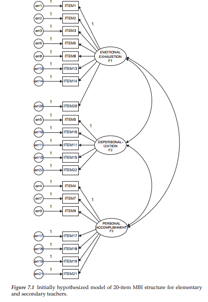
In my preliminary single-group analyses reported in Byrne (1993), I found that, for each teacher group, MBI Items 12 and 16 were extremely prob­lematic; these items were subsequently deleted and a model proposed in which only the remaining 20 items were used to measure the underlying construct of burnout.² This 20-item version of the MBI provides the basis for the hypothesized model under test in the determination of the baseline model for each teacher group and is presented schematically in Figure 7.1. If this model fits the data well for both groups of teachers, it will remain the hypothesized model under test for equivalence across the two groups. On the other hand, should the hypothesized model of MBI structure exhibit a poor fit to the data for either elementary or secondary teachers, it will be modified accordingly and become the hypothesized multigroup model under test. We turn now to this requisite analysis.

Establishing Baseline Models: The General Notion

Because the estimation of baseline models involves no between-group constraints, the data can be analyzed separately for each group. However, in testing for invariance, equality constraints are imposed on particular parameters and, thus, the data for all groups must be analyzed simul­taneously to obtain efficient estimates (Bentler, 2005; Joreskog & Sorbom, 1996a); the pattern of fixed and free parameters nonetheless remains con­sistent with the baseline model specification for each group.³ However, it is important to note that because measurement scales are often group-specific in the way they operate, it is possible that these baseline models may not be completely identical across groups (see Bentler, 2005; Byrne, Shavelson, & Muthen, 1989). For example, it may be that the best-fitting model for one group includes an error covariance (see, e.g., Bentler, 2005) or a cross-loading (see, e.g., Byrne, 1988b, 2004; Reise, Widaman, & Pugh, 1993) whereas these parameters may not be specified for the other group. Presented with such findings, Byrne et al. (1989) showed that by imple­menting a condition of partial measurement invariance, multigroup analyses can still continue. As such, some but not all measurement parameters are constrained equal across groups in the testing for structural equivalence or latent factor mean differences. It is important to note, however, that over the intervening years, the concept of partial measurement equiva­lence has sparked a modest debate in the technical literature (see Millsap & Kwok, 2o04; Widaman & Reise, 1997). Nonetheless, its application remains a popular strategy in testing for multigroup equivalence and is especially so in the area of cross-cultural research. The perspective taken in this book is consistent with our original postulation that a priori know­ledge of major model specification differences is critical to the application of invariance-testing procedures.

Establishing the Baseline Models: Elementary and Secondary Teachers

In testing for the validity of item scores related to the proposed 20-item MBI model for each teacher group, findings were consistent across panels in revealing exceptionally large error covariances between Items 1 and 2, and between Items 5 and 15. As was discussed in Chapter 4, these error covariances can reflect overlapping content between each item pair. Although overlap between Items 1 and 2 was also problematic with the narrower sample of elementary male teachers (see Chapter 4), its presence here with respect to the much larger samples of elementary and secondary teachers (no gender split) further substantiates the troublesome nature of these two MBI items, both of which are designed to measure emotional exhaustion. Item 1 expresses the notion of feeling emotionally drained from one’s work; Item 2 talks about feeling used up at the end of the day. Clearly, these two items appear to be expressing the same idea, albeit the wording has been slightly modified. In a similar manner, Items 5 and 15, both designed to measure depersonalization, showed the same overlap­ping effects for the gender-free full sample of elementary and secondary teachers. Item 5 asks the respondent to reflect on the extent to which he or she treats some students as impersonal objects, while Item 15 taps into the feeling of not caring what happens to some students.⁴

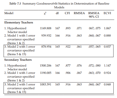
Because many readers may wish to replicate these analyses based on the same data found on the publisher’s website (www.routledge .com/9781138797031), I consider it worthwhile to discuss briefly the findings pertinent to each group of teachers. We turn first to the elemen­tary teachers. With a modification index (MI) of 189.195 and a parameter change statistic (PCS) of .466, it is clear that the error covariance between Items 1 and 2 represents a major model misspecification. Likewise, the same situation holds for the error covariance involving Items 5 and 15 (MI = 56.361; PCS = .284),^s albeit somewhat less dramatically. In addition, based on Model 3 in which the two previous error covariances were speci­fied, results revealed an MI value of 44.766 and a PCS value of .337 related to an error covariance between Items 5 and 6. Although these values are relatively high and close to those for the error covariance between Items 5 and 15, support for their specification is more difficult to defend sub­stantively. Item 6, designed to measure Emotional Exhaustion, relates to stress incurred from working with people all day. In contrast, Item 5 is designed to measure Depersonalization and taps into the sense that the teacher feels he/she treats some students as if they are impersonal objects. Given an obvious lack of coherence between these two items, I do not con­sider it appropriate not to add the error covariance between Items 5 and 6 to the model.

Let’s turn now to the results for secondary teachers. Consistent with findings for elementary teachers, the initial test of the hypothesized model revealed excessively large MI (276.497) and PCS (.522) values representing an error covariance between Items 1 and 2. Likewise, results based on a test of Model 2 yielded evidence of substantial misspecification involving an error covariance between Items 5 and 15 (MI = 99.622; PCS = .414). In contrast to elementary teachers, however, results did not suggest any mis- specification between the error terms related to Items 5 and 6. Nonetheless, an MI value of 45.104 related to an error covariance between Items 7 and 21 called for examination. Given the relatively small value of the PCS (.225), together with the incompatibility of item content, I dismissed the specifi­cation of this parameter in the model. Both items are designed to measure Personal Accomplishment. Whereas Item 7 suggests that the respondent deals effectively with student problems, Item 21 suggests that he or she deals effectively with emotional problems encountered in work. Although the content is somewhat similar from a general perspective, I contend that the specificity of Item 21 in targeting emotional problems argues against the specification of this parameter.

Although these modifications to the initially hypothesized model of MBI structure resulted in a much better-fitting model for both ele­mentary teachers (x²(₁₆₅) = 878.954; CFI = .922; RMSEA = .061) and sec­ondary (x²(₁₆₅) = 1083.39; CFI = .92; RMSEA = .06), the fit nonetheless, was modestly good at best. However, in my judgment as explained above, it would be inappropriate to incorporate further changes to the model. As always, attention to parsimony is of utmost importance in SEM and this is especially true in tests for multigroup equivalence. The more an originally hypothesized model is modified at this stage of the analyses, the more difficult it is to determine measurement and structural equivalence. Goodness-of-fit statistics related to the determi­nation of the baseline models for each teacher group are summarized in Table 7.1.

Findings from this testing for a baseline model ultimately yielded one that was identically specified for elementary and secondary teach­ers. However, it is important to point out that just because the revised model was similarly specified for each teacher group, this fact in no way guarantees the equivalence of item measurements and underlying theor­etical structure; these hypotheses must be tested statistically. For example, despite an identically specified factor loading, it is possible that, with the imposition of equality constraints across groups, the tenability of invari­ance does not hold; that is, the link between the item and its target factor differs across the groups. Such postulated equivalencies, then, must be tested statistically.

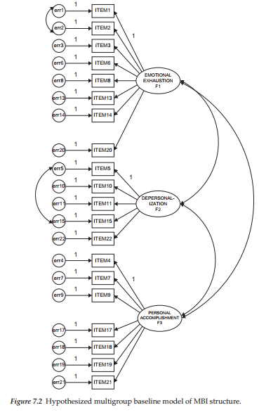
As a consequence of modifications to the originally hypothesized 20-item MBI structure in the determination of baseline models, the hypoth­esized model under test in the present example is the revised 20-item MBI structure as schematically depicted in Figure 7.2. At issue is the extent to which its factorial structure is equivalent across elementary and second­ary teachers. More specifically, we test for the equivalence of the factor loadings (measurement invariance) and factor covariances (structural invariance) across the teaching panels. In addition, it is instructive to test for cross-group equivalence of the two error covariances as this informa­tion reflects further on the validity of these particular items.

4. Modeling with Amos Graphics

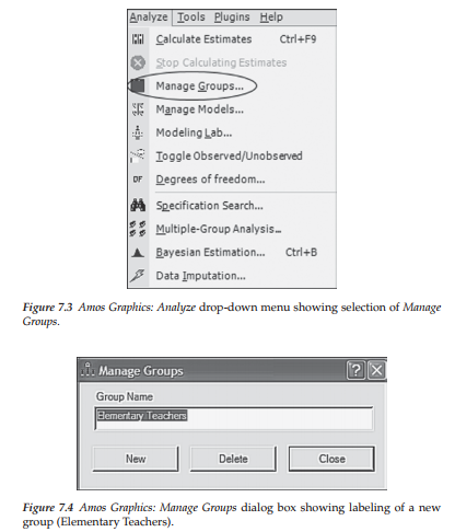
When working with analysis of covariance structures that involve mul­tiple groups, the data related to each must of course be made known to the program. Typically, for most SEM programs, the data reside in some external file, the location of which is specified in an input file. In contrast, however, given that no input file is used with the graphical approach to Amos analyses, both the name of each group and the location of its data file must be communicated to the program prior to any analyses involv­ing multiple groups. This procedure is easily accomplished via the Manage Groups dialog box which, in turn, is made available by pulling down the Analyze menu and selecting the “Manage Groups” option as shown in Figure 7.3. Once you click on this option, you will be presented with the Manage Groups dialog box shown in Figure 7.4. However, when first pre­sented, the text you will see in the dialog box will be “Group Number 1”. To indicate the name of the first group, click on New and replace the former text with the group name as shown for Elementary Teachers in Figure 7.4. Clicking on New again yields the text “Group number 2”, which is replaced by the name “Secondary Teachers.” With more than two groups, each click produces the next group number and the process is repeated until all groups have been identified.

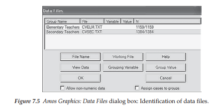
Once the group names have been established, the next task is to iden­tify a data file for each. This procedure is the same as the one demon­strated earlier in the book for single groups, the only difference being that a filename for each group must be selected. The Data File dialog box for the present application that includes information related to both elementary (N = 1,159) and secondary (N = 1,384) teachers is shown in Figure 7.5.

Finally, specification of multigroup models in Amos Graphics is guided by several basic default rules. One such default is that all groups in the analysis will have the identical path diagram structure, unless explicitly declared otherwise. As a consequence, a model structure needs only to be drawn for the first group; all other groups will have the same structure by default. Thus, the hypothesized multigroup model shown in Figure 7.2 represents the one to be tested for its invariance across elementary and secondary teachers. On the other hand, should the baseline models be shown to differ in some way for each group, specific precautions that address this situation must be taken (for an example of this type of Amos application, see Byrne, 2004).

5. Hierarchy of Steps in Testing Multigroup Invariance

5.1. Testing for Configural Invariance

The initial step in testing for multigroup equivalence requires only that the same number of factors and their loading pattern be identical across groups. As such, no equality constraints are imposed on any of the param­eters. Thus, the same parameters that were estimated in the baseline model for each group separately are again estimated, albeit within the framework of a multigroup model. In essence, then, you can think of the model tested here as a multigroup representation of the baseline models. In the present case, then, it incorporates the baseline models for elemen­tary and secondary teachers within the same file. Based on the early work of Horn, McArdle, and Mason (1983), this model is termed the configural model. Unlike subsequent models to be tested, of primary interest here is the extent to which the configural model fits the multigroup data. Model fit statistics consistent with, or better than, those found for each of the groups separately support the claim that the same configuration of esti­mated parameters holds across the groups. More specifically, the number of factors, the pattern of factor loadings, the specified factor covariances, and, in the present case, the two specified error covariances are considered to hold across elementary and secondary teachers. Although no equality constraints are ever specified in testing the configural model, this min­imal test of multigroup model fit can be considered to represent a test for configural invariance.

Given that this model comprises the final best-fitting baseline model for each group, it is expected that results will be indicative of a well-fitting model. Importantly, however, it should be noted that despite evidence of good fit to the multi-sample data, the only information that we have at this point is that the factor structure is similar, but not necessarily equiva­lent across groups. Given that no equality constraints are imposed on any parameters in the model, no determination of group differences related to either the items or the factor covariances can be made. Such claims derive from subsequent tests for invariance to be described shortly.

Because we have already conducted this test in the establishment of baseline models, you are no doubt wondering why it is necessary to repeat the process. Indeed, there are two important reasons for doing so. First, it allows for the simultaneous testing for invariance across the two groups. That is, the parameters are estimated for both groups at the same time. Second, in testing for invariance, the fit of this configural model pro­vides the baseline value against which all subsequently specified invari­ance models are compared. Despite the multigroup structure of this and subsequent models, analyses yield only one set of fit statistics for overall model fit. When ML estimation is used, the x² statistics are summative and, thus, the overall x² value for the multigroup model should equal the sum of the x² values obtained when the baseline model is tested separately for each group of teachers.⁶ Consistent with the earlier single-group analy­ses, goodness-of-fit for this multigroup model should exhibit a good fit to the data for the dual group parameterization. Realistically, however, these multigroup fit statistics can never be better than those determined for each group separately. Thus, in light of only modestly good fit related to the baseline model for both elementary and secondary teachers, we cannot expect to see better results for this initial multigroup model.

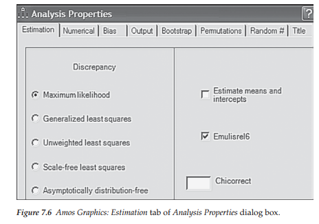
Before testing for invariance related to the configural model, I addressed the caveat raised in Note 6 and checked the “Emulisrel6” option listed on the Estimation tab of the Analysis Properties dialog box, illustrated in Figure 7.6. Because the Amos output file for multigroup models may seem a little confusing at first, I now review selected portions as they relate to this initial model.

Selected Amos Output: The Configural Model (No Equality Constraints Imposed)

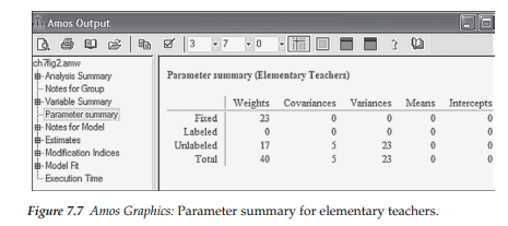
Although the overall output definitely relates to the multigroup model, the program additionally provides separate information for each group under study. Because the basic output format for single group analyses has been covered earlier in the book, I limit my review here to the Parameter summary as it pertains only to elementary teachers. All other portions of the output focus on results for the two groups in combination. Let’s turn first to Figure 7.7, which focuses on the parameter summary.

Parameter summary. In reviewing Figure 7.7, you will see the usual text output tree in the narrow column on the left, from which you can select the portion of the output you wish to review. Not shown here due to space restrictions, is the continuation of this vertical column where both group names are listed. Simply clicking on the group of interest provides the correct parameter information pertinent to the one selected. Given that I clicked on Elementary Teachers before selecting Parameter Summary from the output file tree, I was presented with the content shown in Figure 7.7; clicking on Secondary Teachers, of course, would yield results pertinent to that group. In this section of the output file, Amos focuses on fixed and freely estimated parameters, the latter being further classified as “Labeled” and “Unlabeled.” Labeled parameters are those that are con­strained equal to another group or parameter. Specifying equality con­straints related to parameters was detailed in Chapter 5; specification for groups will be covered later in this chapter. Because no constraints have been imposed in this configural model, the output text shows zero labeled parameters. The only relevant parameters for this model are the regres­sion paths representing the factor loadings (termed “Weights”), variances, and covariances, all of which are freely estimated.

Turning to results for the regression paths, we note that 23 are fixed, and 17 are freely estimated. The fixed parameters represent the 20 regres­sion paths associated with the error terms, in addition to the three factor regression paths fixed to 1.00 for purposes of model identification; the 17 unlabeled parameters represent the estimated factor loadings. Continuing through the remainder of the table, the five covariances represent rela­tions among the three factors plus the two error covariances. Finally, the 23 variances refer to the 20 error variances in addition to the three fac­tor variances. In total, the number of parameters specified for Elementary Teachers is 68, of which 23 are fixed, and 45 freely estimated. Clicking on the tab for Secondary Teachers reveals the same number of parameters, thereby yielding 136 parameters in total for the hypothesized multigroup MBI model shown in Figure 7.2.

Let’s turn now to Figure 7.8 where degrees of freedom information for the multigroup model is summarized. Under the heading “Computation of degrees of freedom (Your model)” we find three lines of information. The first line relates to the number of sample moments (i.e., number of elements in the combined covariance matrices). In Chapter 2, you learned how to calculate this number for a single group. However, it may be help­ful to review the computation relative to a multigroup application. Given that there are 20 observed variables (i.e., 20 items) in the hypothesized model, we know that, for one group, this would yield 210 ([20 x 21]/2) pieces of information (or, in other words, sample moments). Thus, for two groups, this number would be 420 as shown in this part of the output file.

Line 2 in Figure 7.8 relates to the number of estimated parameters in the model. In Figure 7.7, we observed that this number (for elemen­tary teachers) was 45 (17 + 5 + 23). Taking into account both groups, then, we have 90 estimated parameters. Degrees of freedom are reported on line 3 to be 330. Given 420 sample moments and 90 estimated parameters, this leaves us with 420 – 90 = 330 degrees of freedom. (For a review and explanation of these calculations, see Chapter 2.)

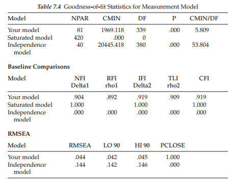
Model assessment. Let’s turn now to Table 7.2 in which the goodness-of- fit statistics for this multigroup model are reported. The key values to note are those of the x²-statistic, the CFI, and the RMSEA; the ECVI value is irrelevant in this context.

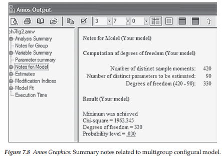
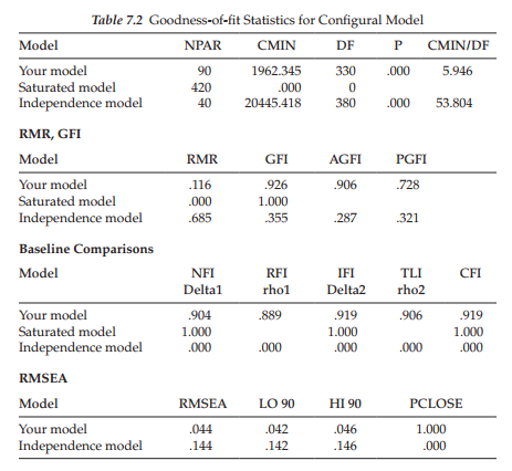
Results related to this first multigroup model testing for configural invariance, reveal the x² value to be 1,962.345 with 330 degrees of freedom. The CFI and RMSEA values, as expected, are .919 and .044, respectively. From this information, we can conclude that the hypothesized multigroup model of MBI structure is modestly well-fitting across elementary and sec­ondary teachers.

Having established goodness-of-fit for the configural model, we now proceed in testing for the invariance of factorial measurement and struc­ture across groups. However, because you need to know the manner by which tests for invariance are specified using Amos Graphics before try­ing to fully grasp an understanding of the invariance testing process in and of itself, I present this material in two parts. First, I introduce you to two different approaches to testing for multigroup invariance using Amos—manual versus automated. I then walk you through a test for invariance of the hypothesized multigroup model (see Figure 7.2) across elementary and secondary teachers within the framework of the manual approach. Application of the automated approach to testing for multi­group invariance is discussed and illustrated in Chapters 8 and 9.

5.2. Testing for Measurement and Structural Invariance: The Specification Process

In testing for configural invariance, interest focused on the extent to which the number of factors and pattern of their structure were simi­lar across elementary and secondary teachers. In contrast, in testing for measurement and structural invariance, interest focuses more specific­ally on the extent to which parameters in the measurement and struc­tural components of the model are equivalent across the two groups. This testing process is accomplished by assigning equality constraints on particular parameters (i.e., the parameters are constrained equal across groups). The procedure operates in such a way that these parameters are estimated for the first group only; estimates for all remaining groups are constrained equal to those of the first group. In Amos Graphics, con­straints can be specified via two approaches: (a) individually assigning a label to each parameter to be held equal across groups, and (b) using the automated models of parameter subsets contained in the Multiple Group dialog box. Although any parameters that are unlabeled will be freely estimated using the manual approach to invariance specification, this dictum does not hold for the automated approach. Despite the specifi­cation of selected parameters as freely estimated, their assigned labels remain on the graphical representation of the model, albeit the related parameters are freely estimated (J. Arbuckle, personal communication, June 7, 2008). I begin by introducing you to the manual labeling approach to specification of equality constraints and then follow with the auto­mated approach.

The manual multiple group approach. In testing for invariance, my prefer­ence is to follow the classical approach, which entails first running a model in which only the factor loadings are constrained equal (i.e., measurement model). Provided with evidence of group equivalence, these factor loading parameters remain constrained and equality constraints are then placed on the factor variances and covariances (i.e., structural model). Although error variances associated with each of the observed variable items are also part of the measurement model, testing for their equality across groups is con­sidered to be excessively stringent and therefore is rarely implemented. On the other hand, in our testing for the validity of the MBI, we deter­mined two very strong and group-consistent error covariances. For both statistical and substantive reasons, I consider it important to include these particular error parameters in our test for invariance of the measurement model. First, each error covariance was found to be excessively large in both groups. Second, scrutiny of the related items revealed highly over­lapping content across each aberrant pair of items. Such redundancy can reflect itself in the form of error covariation. Taking these two perspectives into account, it seems prudent to ascertain whether the two error covari­ance parameters hold across teaching panels as such evidence speaks to the problematic nature of the content related to these MBI items.

Specification of equality constraints using the manual approach entails two related steps. It begins by first clicking on the parameter you wish to label and then right-clicking on the mouse to produce the Object Properties dialog box (illustrated in previous chapters). Once this box is opened, the Parameter tab is activated and then the label entered in the space provided in the bottom left corner. This process is graphically shown in Figure 7.9 as it relates to the labeling of the second factor regression path represent­ing the loading of Item 2 on Factor 1 (Emotional Exhaustion). Once the cursor is clicked on the selected parameter, the latter takes on a red color. Right-clicking the mouse subsequently opens the Object Properties dialog box where you can see that I have entered the label “L2” in the lower left corner under the heading Regression weight. The second part of this initial step requires that you click on the “All groups” box (shown within the ellipse in Figure 7.9). Checking this box tells the program that the param­eter applies to both groups.⁷

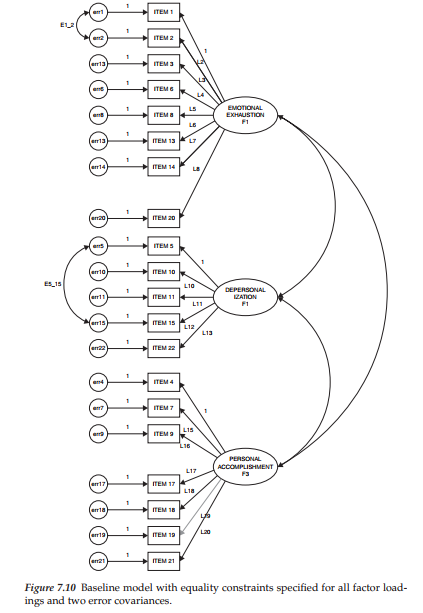
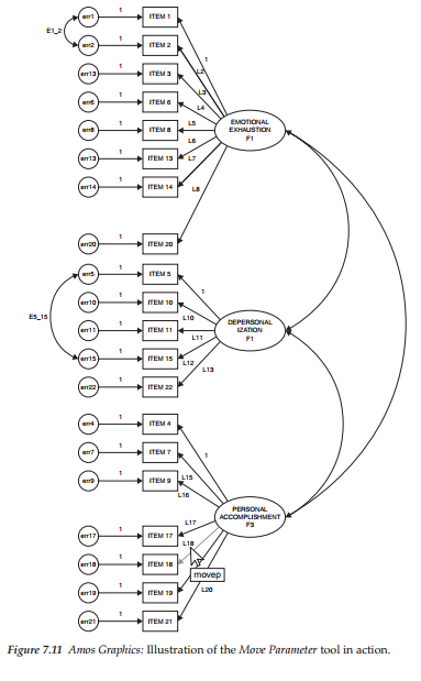
Turning to Figure 7.10, you will see the factor loadings and two error covariances of the hypothesized model labeled and ready for a statistical testing of their invariance. However, three aspects of Figure 7.10 are note­worthy. First, selected labeling of parameters is purely arbitrary. In the present case, I chose to label the factor loading regression paths as L. Thus, L2, for example, represents the loading of Item 2 on Factor 1. Second, you will note that the value of 1.00, assigned to the first of each congeneric set of indicator variables, remains as such and has not been relabeled with an “L.” Given that this parameter is already constrained to equal 1.00, its value will be constant across the two groups. Finally, the somewhat erratic labeling of the factor loading paths is a function of the automated labeling process provided in Amos. Although, technically, it should be possible to shift these labels to a more appropriate location using the Move Parameter tool (n), this transition does not work well when there are several labeled parameters located in close proximity to one another, as is the case here. This malfunction appears to be related to the restricted space allotment assigned to each parameter. To use the Move Parameters tool, click either on its icon in the toolbox, or on its name from the Edit drop-down menu. Once this tool is activated, point the cursor at the parameter you wish to move; the selected parameter will then take on a red color. Holding the left mouse button down simply move the parameter label to another location.

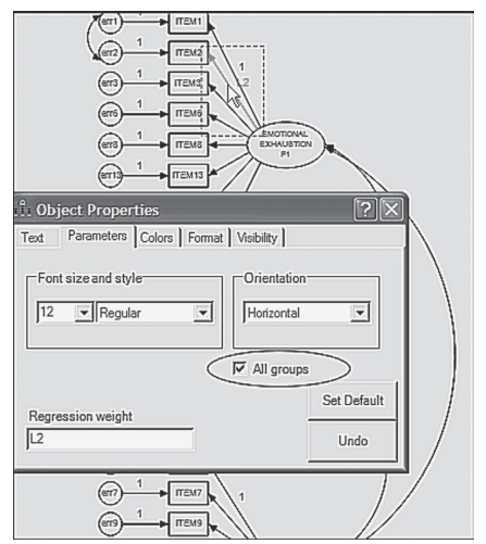
Figure 7.9 Amos Graphics: Object Properties dialog box showing labeling of parameter

This process is illustrated in Figure 7.11 as it relates to factor loading 18 (L18) representing Item 18.

As labeled, the hypothesized multigroup model in Figure 7.10 speci­fies the following parameters to be tested for group invariance: (a) 17 fac­tor loadings, and (b) 2 error covariances (Items 1 and 2; Items 5 and 15).

Because the automated multiple approach to tests for invariance pre­sents a fully labeled model by default (i.e., labeling associated with the factor loadings, variances, and covariances as well as the error variances),

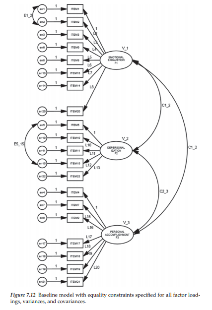
I additionally include here a model in which the factor variances and covariances, as well as the factor loadings and two error covariances, are postulated to be invariant (see Figure 7.12).

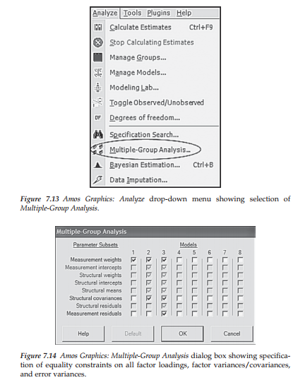
The automated multiple-group approach. This procedure is activated by either clicking on the Multiple Group icon ffff), or by pulling down the Analyze menu and clicking on Multiple-Group Analysis as shown in Figure 7.13. Either action automatically produces the Multiple-Group Analysis dialog box shown in Figure 7.14.

On the left side of this dialog box you will see a list of parameter sub­sets, and along the top, a series of eight numbers under each of which is a column of small squares. The darkest checkmarks that you see in the dialog box are default and represent particular models to be tested. When the dialog box is first opened, you will observe the three defaulted models shown in Figure 7.14. The checkmark in the first column (identified as “1”) indicates a model in which only the factor loadings (i.e., measure­ment weights) are constrained equal across groups (Model 1). Turning to Columns 2 and 3, we see both dark and grayed checkmarks. The darkest checkmarks in Column 2 indicate a model in which all estimated factor loadings, as well as factor variances and covariances (i.e., structural covar­iances), are constrained equal across groups (Model 2); those in Column 3 represent a model having all estimated factor loadings, factor variances, factor covariances, and error variances (i.e., measurement residuals) con­strained equal across groups (Model 3). The grayed checkmarks in both columns represent parameter subsets that may be included in the testing of additional models.

Relating this approach to the checked dialog box shown in Figure 7.14, would be tantamount to testing Model 1 first, followed by a test of Model 2 as exemplified in Figures 7.10 and12 for the manual approach to invariance. This process can continue with the addition of other param­eter subsets, as deemed appropriate in testing any particular multigroup model. An important point to note in using Amos Graphics, however, is the automated checkmarks related to Model 3. As noted earlier, measure­ment error variances are rarely constrained equal across groups as this parameterization is considered to be an excessively stringent test of mul­tigroup invariance. Thus, the testing of Model 3 is relatively uncommon. However, one example of where Model 3 would be important is when a researcher is interested in testing for the equality of reliability related to an assessment scale across groups (see, e.g., Byrne, 1988a).

Although it was mentioned briefly in the introduction of this section, I consider it important to note again a major model specification aspect of this automated approach as currently implemented in Amos (Version 23). Once you select the Multiple Groups option, Amos automatically labels all parameters in the model whether or not you wish to constrain them equal across groups. For example, although we do not wish to test a mul­tigroup model in which all error variances are postulated to be invariant across groups (Model 3), all labeling on the graphical model with respect to these parameters remains intact even though we wish not to have equality constraints on these parameters. Removal of these checkmarks (for Model 3) is easily accomplished by simply clicking on them. Although these error variances subsequently will not be estimated, the labeling of these parameters nonetheless remains on the “behind-the-scenes” work­ing Amos model.

5.3. Testing for Measurement and Structural Invariance:

Model Assessment

As noted earlier, one major function of the configural model is that it provides the baseline against which all subsequent tests for invariance are compared. In the Joreskog tradition, the classical approach in argu­ing for evidence of noninvariance is based on the x²-difference (Ay²) test (see Chapter 4, Note 7). The value related to this test represents the differ­ence between the x² values for the configural and other models in which equality constraints have been imposed on particular parameters. This difference value is distributed as x² with degrees of freedom equal to the difference in degrees of freedom. Evidence of noninvariance is claimed if this x²-difference value is statistically significant. The researcher then follows up with additional tests aimed at targeting which parameters are accounting for these noninvariant findings. This procedure is demon­strated in the testing of both measurement and structural equivalence of the MBI in this chapter.

Over the past decade or so, applied researchers have argued that from a practical perspective, the x²-difference test represents an exces­sively stringent test of invariance and particularly in light of the fact that SEM models at best are only approximations of reality (Cudeck & Brown 1983; MacCallum et al., 1992). Consistent with this perspective, Cheung and Rensvold (2002) reasoned that it may be more reasonable to base invariance decisions on a difference in CFI (ACFI) rather than on x² values. Thus, based on a rigorous Monte Carlo study of several goodness-of-fit indices, Cheung and Rensvold (2002) proposed that evi­dence of noninvariance be based on a difference in CFI values exhibit­ing a probability <0.01. Building upon this earlier investigative work of Cheung and Rensvold, Chen (2007) sought to examine the sensitivity of goodness-of-fit indices to lack of measurement invariance as they relate to factor loadings, intercepts, and error (or residual) variances. Based on two Monte Carlo studies, Chen found the SRMR to be more sensitive to lack of invariance with respect to factor loadings than for intercepts and error variances. In contrast, the CFI and RMSEA were found to be equally sensitive to all three types of noninvariance. Although Chen addition­ally suggested revised cutoff values for the CFI- difference test, these recommended values vary for the SRMR and RMSEA, as well as for sam­ple size. In reviewing results pertinent to tests for invariance of the MBI in this chapter, we will examine results derived from the x²-difference test, as well as the CFI-difference test based on the cutoff value recom­mended by Cheung and Rensvold (2002).

6. Testing For Multigroup Invariance:

The Measurement Model

Now that you are familiar with the procedural steps conducted in testing for multigroup invariance, as well as with the two approaches to imple­mentation of these procedures made available in Amos Graphics, we now move on to actual implementation of these procedures as outlined earlier. In this chapter, we focus on only the manual approach to invariance test­ing; Chapters 8 and 9 address the automated approach.

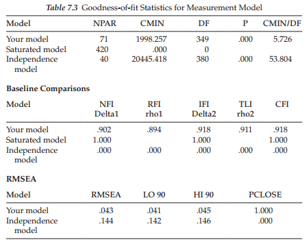
Turning to the task at hand here, we examine results related to the labeled model shown in Figure 7.10. You will recall that this model (which we’ll call Model A to distinguish it from subsequently specified models as well as to simplify the comparison of models), tests for the equivalence of all factor loadings plus two error covariances (Items 1 and 2; Items 5 and 15). Let’s turn now to these results, which are sum­marized in Table 7.3.

Model Assessment

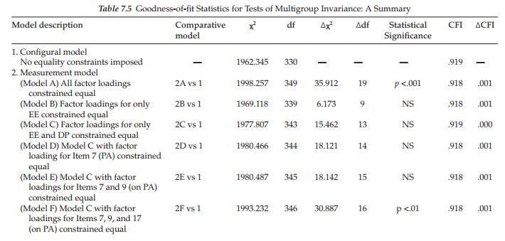
A review of these results, as expected, reveals the fit of this model to be consistent with that of the configural model (CFI = .918; RMSEA = .043). However, of prime importance in testing for invariance of the factor loadings and two error covariances are results related to the x²– and CFI-difference tests. As noted earlier, computation of these results involves taking their differences from the x² and CFI values reported for the con­figural model (see Table 7.2), which yields the following: Ax²(₁₉) = 35.912 and ACFI = .001. Not surprisingly, given its statistical stringency, the X²-difference test argues for evidence of noninvariance, whereas the CFI-difference test argues for invariance. That the Ax²-difference test is said to argue for noninvariance is based on the finding that a x² value of 35.912, with 19 degrees of freedom, is shown on the x² distribution table to be statistically significant at a probability value <.01. On the other hand, the ACFI value of .001 contends that the measurement model is completely invariant in that this value is less than the .01 cutoff point proposed by Cheung and Rensvold (2002).

Presented with these divergent findings, the decision of which one to accept is purely an arbitrary one and rests solely with each individual researcher. It seems reasonable to assume that such decisions might be based on both the type of data under study and/or the circumstances at play. For our purposes here, however, I consider it worthwhile to focus on the Ay² results as it provides me with the opportunity to walk you through the subsequent steps involved in identifying which parameters in the model are contributing to these noninvariant findings; we press on then with the next set of analyses.

In testing for multigroup invariance, it is necessary to establish a logically organized strategy, the first step being a test for invariance of all factor loadings, which we have now completed. Given findings of nonin­variance at this level, we then proceed to test for the invariance of all fac­tor loadings comprising each subscale (i.e., all loadings related to the one particular factor), separately. Given evidence of noninvariance at the sub­scale level, we then test for the invariance of each factor loading (related to the factor in question), separately. Of import in this process is that, as factor loading parameters are found to be invariant across groups, their specified equality constraints are maintained, cumulatively, throughout the remainder of the invariance-testing process.

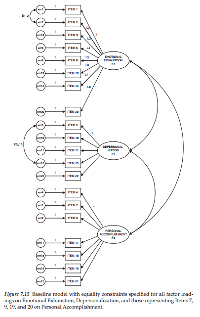
Having determined evidence of noninvariance when all factor load­ings are held equal across groups, our next task is to test for the invariance of factor loadings relative to each subscale separately. This task is easily accomplished in Amos Graphics through a simple modification of the exist­ing labeled model shown in Figure 7.10. As such, we remove all factor load­ing labels, except those associated with Emotional Exhaustion (Factor 1), simply by clicking on each label (to be deleted), right-clicking in order to trigger the Object Properties dialog box, and then deleting the label listed in the parameter rectangle of the dialog box (see Figure 7.9). Proceeding in this manner presents us with the labeled model (Model B) displayed in Figure 7.15; all unlabeled parameters will be freely estimated for both elementary and secondary teachers.

Turning to Table 7.4, we see that the testing of Model B yielded a x² value of 1969.118 with 339 degrees of freedom. This differential of nine degrees of freedom derives from the equality constraints placed on seven factor loadings (the first loading is already fixed to 1.0) plus the two error covariances. Comparison with the configural model yields a Ax²(₉) value of 6.173, which is not statistically significant.

These findings advise us that all items designed to measure Emotional Exhaustion are operating equivalently across the two groups of teach­ers. Our next task then is to test for the equivalence of items measuring Depersonalization. Accordingly, we place equality constraints on all freely estimated factor loadings associated with Factor 2, albeit at the same time, maintaining equality constraints for Factor 1 (Model C). Again, this spe­cification simply means a modification of the model shown in Figure 7.15 in that labels are now added to the four estimated factor loadings for Depersonalization.

Because you are now familiar with the process involved in labeling these models and in the interest of space, no further figures or separate tables are presented for models yet to be tested. Results for these subse­quent models are summarized in Table 7.5.

As reported in Table 7.5, the test of Model C yielded a x² value of 1977.807 with 343 degrees of freedom; the additional four degrees of freedom derive from the equality constraints placed on the four estimated factor loadings for Factor 2. These results therefore yielded a Ax²(₁₃) value of 15.462, which once again is statistically nonsignificant. Provided with this information, we now know that the problematic items are housed in the subscale designed to measure Personal Accomplishment. Accordingly, we proceed by labeling (on the model) and testing one factor loading at a time within this subscale. Importantly, provided with evidence of nonsignificance related to a single factor loading, this invariant loading is held constrained during subsequent tests of the remaining items. Results related to these individual loadings are discussed as a group and reported in Table 7.5.

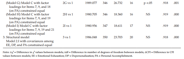
In reviewing these tests of individual factor loadings measuring Factor 3, Personal Accomplishment, findings reveal evidence of noninvariance related to two items—Item 17 (p < .01) and Item 18 (p < .05) (see results for measurement models F and G). Item 17 suggests that the respondent is able to create a relaxed atmosphere with his/her students and Item 18 conveys the notion that a feeling of exhilaration follows from working closely with students. From these findings we learn that, for some reason, Items 17 and 18 are operating somewhat differently in their measurement of the intended content for elementary and secondary teachers. The task for the researcher confronted with these noninvariant findings is to pro­vide possible explanations of this phenomenon.

Before moving on to a test of structural invariance, I consider it important to further clarify results reported in Table 7.5 with respect to measurement models F, G, and H. Specifically, it’s important that I explain why each of these models has the same number of degrees of freedom. For Model F, of course, 16 degrees of freedom derives from the fact that we have added an equality constraint for Item 17 over and above the constraints specified in the previous model (Model E). Model G has 16 degrees of freedom because noninvariant Item 17 is now freely estimated with Item 18 constrained in its place. Likewise, Model H has 16 degrees of freedom as Item 19 replaced noninvariant Item 18, which is now freely estimated. Hopefully, this explanation should dear up any questions that you may have had concerning these results.

7. Testing For Multigroup Invariance: The Structural Model

Now that equivalence of the measurement model has been established, the next step in the process is to test for invariance related to the structural portion of the model. Although these tests can involve the factor variances as well as the factor covariances, many researchers consider the latter to be of most interest; I concur with this notion. In particular, testing for the invariance of factor covariances addresses concerns regarding the extent to which the theoretical structure underlying the MBI (in this case) is the same across groups.

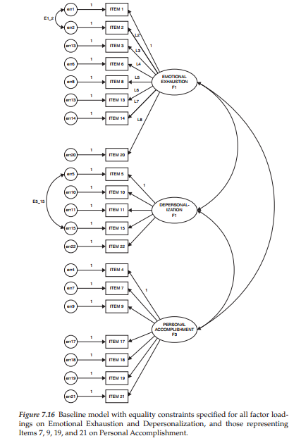
In this part of the testing process, the model specifies all factor load­ings except those for Items 17 and 18, in addition to the three factor covariances constrained equal across elementary and secondary teachers. Given that these two items were found to be noninvariant, they are freely estimated, rather than held constrained equal across groups. As such, the model now represents one that exhibits partial measurement invari­ance. This final model is presented in Figure 7.16. Given the rather poor labeling mechanism for this model, I show the two noninvariant factor loadings for Items 17 and 18 encased in a broken-line oval; the fact that their factor loading regression paths are not labeled ensures that they are freely estimated. Results for this test of structural invariance, as reported in Table 7.5, revealed the factor covariances to be equivalent across elem­entary and secondary teachers.

Source: Byrne Barbara M. (2016), Structural Equation Modeling with Amos: Basic Concepts, Applications, and Programming, Routledge; 3rd edition.