Application 6: Testing Invariance of Latent Mean Structures (First-Order CFA Model) with AMOS

1. Key Concepts

• Distinguishing between observed and latent means
• Distinguishing between covariance and mean structures
• The moment matrix
• Critically important constraints regarding model identification and factor identification
• Illustrated use of the automated multigroup procedure in testing invariance
• Link between multigroup dialog box and automated labeling of Amos graphical models

In the years since the printing of my first Amos book (Byrne, 2001) there has been a steady, yet moderate increase in reported findings from tests for multigroup equivalence. A review of the SEM literature, however, reveals most tests for invariance to have been based on the analysis of covariance structures (COVS), as exemplified in Chapter 7 of this volume. Despite Sorbom’s (1974) introduction of the mean and covariance struc­tures (MACS) strategy in testing for latent mean differences over 40 years ago, only a modicum of studies have been designed to test for latent mean differences across groups based on real (as opposed to simulated) data (see, e.g., Aiken, Stein, & Bentler, 1994; Byrne, 1988b; Byrne & Stewart, 2006; Little, 1997; Marsh & Grayson, 1994; Cooke, Kosson, & Michie, 2001; Reise et al. 1993; Widaman & Reise, 1997). The aim of this chapter, then, is to introduce you to basic concepts associated with the analysis of latent mean structures, and to walk you through an application that tests for their invariance across two groups. Specifically, we test for differences in the latent means of general, academic, English, and mathematics self-concepts across high- and low-track secondary school students. The example pre­sented here draws from two published papers—one that focuses on meth­odological issues related to testing for invariant covariance and mean structures (Byrne et al., 1989), and one oriented toward substantive issues related to social comparison theory (Byrne, 1988b).

2. Basic Concepts Underlying Tests of Latent Mean Structures

In the usual univariate or multivariate analyses involving multigroup comparisons, one is typically interested in testing whether the observed means representing the various groups are statistically significantly dif­ferent from each other. Because these values are directly calculable from the raw data, they are considered to be observed values. In contrast, the means of latent variables (i.e., latent constructs) are unobservable; that is, they are not directly observed. Rather, these latent constructs derive their structure indirectly from their indicator variables which, in turn, are dir­ectly observed and hence, measurable. Testing for the invariance of mean structures, then, conveys the notion that we intend to test for the equiva­lence of means related to each underlying construct or factor. Another way of saying the same thing, of course, is that we intend to test for differences in the latent means (of factors for each group).

For all the examples considered thus far, the analyses have been based on covariance structures. As such, only parameters representing regression coefficients, variances, and covariances have been of interest. Accordingly, the covariance structure of the observed variables consti­tutes the crucial parametric information; a hypothesized model can thus be estimated and tested via the sample covariance matrix. One limitation of this level of invariance is that while the unit of measurement for the underlying factors (i.e., the factor loading) is identical across groups, the origin of the scales (i.e., the intercepts) is not. As a consequence, com­parison of latent factor means is not possible, which led Meredith (1993) to categorize this level of invariance as “weak” factorial invariance. This limitation, notwithstanding, evidence of invariant factor loadings none­theless permits researchers to move on in testing further for the equiva­lence of factor variances, factor covariances, and the pattern of these factorial relations, a focus of substantial interest to researchers interested more in construct validity issues than in testing for latent mean differ­ences. These subsequent tests would continue to be based on the analysis of covariance structures.

In contrast, when analyses are based on mean and covariance struc­tures, the data to be modeled include both the sample means and the sam­ple covariances. This information is typically contained in a matrix termed a moment matrix. The format by which this moment matrix is structured, however, varies with each particular SEM program.

In the analysis of covariance structures, it is implicitly assumed that all observed variables are measured as deviations from their means; in other words, their means (i.e., their intercepts) are equal to zero. As a conse­quence, the intercept terms generally associated with regression equations are not relevant to the analyses. However, when these observed means take on nonzero values, the intercept parameter must be considered thereby necessitating a reparameterization of the hypothesized model. Such is the case when one is interested in testing the invariance of latent mean structures, which necessarily includes testing first for invariance of the observed variable intercepts.

To help you in understanding the concept of mean structures, I draw on the work of Bentler (2005) in demonstrating the difference between covariance and mean structures as it relates to a simple bivariate regres­sion equation. Consider first, the following regression equation:

 y = α + βx + ε(1)

where a is an intercept parameter. Although the intercept can assist in defining the mean of y, it does not generally equal the mean. Now, if we take expectations of both sides of this equation, and assume that the mean of e is zero, the above expression yields

 μy = α + βμx(2)

where  μy is the mean of y, and μ_x is the mean of x. As such, y and its mean can now be expressed in terms of the model parameters a, (, and n_x. It is this decomposition of the mean of y, the dependent variable, that leads to the term mean structures. More specifically, it serves to characterize a model in which the means of the dependent variables can be expressed or “structured” in terms of structural coefficients and the means of the independent variables. The above equation serves to illustrate how the incorporation of a mean structure into a model necessarily includes the new parameters a and iv the intercept and observed mean (of x), respec­tively. Thus, models with structured means merely extend the basic con­cepts associated with the analysis of covariance structures.

In summary, any model involving mean structures may include the following parameters:

• regression coefficients;
• variances and covariances of the independent variables;
• intercepts of the dependent variables;
• means of the independent variables;

Estimation of Latent Variable Means

As with the invariance applications presented in Chapters 7 and 9, this application of a structured means model involves testing simultaneously across two groups.¹ The multigroup model illustrated in this chapter is used when one is interested in testing for group differences in the means of particular latent constructs. This approach to the estimation of latent mean structures was first brought to light in Sorbom’s (1974) seminal extension of the classic model of factorial invariance. As such, testing for latent mean differences across groups is made possible through the implementation of two important strategies—model identification and factor identification.

Model identification. Given the necessary estimation of intercepts associated with the observed variables, in addition to those associated with the unobserved latent constructs, it is evident that the attainment of an overidentified model is possible only with the imposition of sev­eral specification constraints. Indeed, it is this very issue that compli­cates, and ultimately renders impossible, the estimation of latent means in single-group analyses. Multigroup analyses, on the other hand, pro­vide the mechanism for imposing severe restrictions on the model such that the estimation of latent means is possible. More specifically, because two (or more) groups under study are tested simultaneously, evaluation of the identification criterion is considered across groups. As a consequence, although the structured means model may not be identified in one group, it can become so when analyzed within the framework of a multigroup model. This outcome occurs as a function of specified equality constraints across groups. More specifically, these equality constraints derive from the underlying assumption that both the observed variable intercepts and the factor loadings are invariant across groups.

Factor identification. This requirement imposes the restriction that the factor intercepts for one group are fixed to zero; this group then operates as a reference group against which latent means for the other group(s) are compared. The reason for this reconceptualization is that when the intercepts of the measured variables are constrained equal across groups this leads to the latent factor intercepts having no definite origin (i.e., they are undefined in a statistical sense). A standard way of fixing the origin, then, is to set the factor intercepts of one group to zero (see Bentler, 2005; Joreskog & Sorbom, 1996). As a consequence, factor intercepts (i.e., factor means) are interpretable only in a relative sense. That is to say, one can test whether the latent variable means for one group differ from those of another, but one cannot estimate the mean of each factor in a model for each group. In other words, while it is possible to test for latent mean differences between say, adolescent boys and adolescent girls, it is not possible to estimate the mean of each factor for both boys and girls simultaneously; the latent means for one group must be constrained to zero.

Having reviewed the conceptual and statistical underpinning of the mean structures model, I now introduce you to the hypothesized model under study in this chapter.

3. The Hypothesized Model

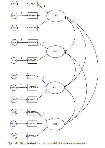
The application to be examined in this chapter addresses equivalency of the latent factor means related to four self-concept (SC) dimensions (gen­eral, academic, English, mathematics) for high (n = 582) and low (n = 248) academically tracked high school students (Byrne, 1988b). The substan­tive focus of the initial study (Byrne, 1988b) was to test for latent mean differences in multidimensional SCs across these two ability groups. This CFA model followed from an earlier study designed to test for the multidi­mensionality of SC (Byrne & Shavelson, 1986) as portrayed schematically in Figure 8.1.

As you will note in the figure, except for Academic SC, the remain­ing dimensions are measured by three indicator variables, each of which represents a subscale score. Specifically, General SC is measured by sub­scale scores derived from the General SC subscale of the Self Description Questionnaire III (SDQIII; Marsh, 1992b), the Affective Perception Inventory (API: Soares & Soares, 1979), and the Self-esteem Scale (SES; Rosenberg, 1965); these indicator variables are labeled as SDQGSC, APIGSC, and SESGSC, respectively. English SC is measured by sub­scale scores related to the SDQIII (SDQESC), the API (APIESC), and the Self-concept of Ability Scale (SCAS; Brookover, 1962), labeled as SCAESC in Figure 8.1. Finally, Math SC is measured by subscale scores derived from the SDQIII (SDQMSC), the API (APIMSC), and the SCAS (SCAMSC). In the case of academic SC, findings from a preliminary factor analysis of the API (see Byrne & Shavelson, 1986) revealed several inadequacies in its measurement of this SC dimension. Thus, it was deleted from all subse­quent analyses in the Byrne & Shavelson (1986) study and the same holds true here.

In contrast to the CFA model discussed in Chapter 7, in which the items of a measuring instrument formed the units of measurement, the CFA model under study in this chapter entails subscale scores of meas­uring instruments as its unit of measurement. It is hypothesized that each subscale measure will have a nonzero loading on the SC factor it is designed to measure albeit a zero loading on all other factors, and that error/uniquenesses associated with each of the observed measures are uncorrelated. Consistent with theory and empirical research, the four SC factors are shown to be intercorrelated.

The Baseline Models

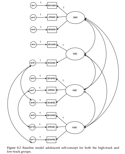
As with the example of multigroup invariance across independent sam­ples in Chapter 7, goodness-of-fit related to the hypothesized model (Figure 8.1) was tested separately for high- and low-track students. Model fit statistics indicated only a modestly well-fitting model for both groups (high-track, CFI = .923, RMSEA = .128; low-track, CFI = .911, RMSEA = .114). Indeed, a review of the modification indices, for both groups, revealed substantial evidence of misspecification as a conse­quence of error covariances among subscales of the same measuring instrument—the SCAS. This finding of overlapping variance among the SCAS subscales is certainly not surprising and can be explained by the fact that items on the English and Math SC subscales were spawned from those comprising the Academic SC subscale. More specifically, the SCAS was originally designed to measure only Academic SC. However, in their attempt to measure the subject-specific facets of English and Math SCs, Byrne and Shavelson (1986) used the same items from the original SCAS, albeit modified the content to tap into the more specific facets of English SC and Math SC.

Given both a substantively and psychometrically reasonable rationale for estimating these three additional parameters, the originally hypoth­esized model was respecified and reestimated accordingly for each group. Testing of these respecified models resulted in a substantially better-fitting model for both high-track (CFI = .975; RMSEA = .076) and low-track (CFI = .974; RMSEA = .065) students. This final baseline model (which turns out to be the same for each group) serves as the model to be tested for its equivalence across high- and low-track students; it is schematically portrayed in Figure 8.2.

4. Modeling with Amos Graphics

The Structured Means Model

In working with Amos Graphics, the estimation and testing of structured means models is not much different from that of testing for invariance based on the analysis of covariance structures. It does, however, require a few additional steps. As with the multigroup application presented in Chapter 7, the structured means model requires a system of labeling whereby certain parameters are constrained to be equal across groups, while others are free to take on any value. In testing for differences in factor latent means, for example, we would want to know that the meas­urement model is operating in exactly the same way for both high- and low-track students. In the structured means models, this requirement includes the observed variable intercepts in addition to the factor loadings (i.e., regression weights) and, thus, both are constrained equal across both groups. We turn now to a more detailed description of this process as it relates to testing for latent mean differences.

5. Testing for Latent Mean Differences

The Hypothesized Multigroup Model

In testing for latent mean differences using Amos Graphics, the base­line model for each ability group must be made known to the program. However, in the case of our academically-tracked groups in this chapter, the final model for each was the same. Thus, the multigroup model shown in Figure 8.2 represents both groups.²

Steps in the Testing Process

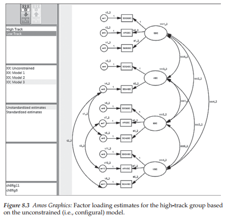
Once the multigroup model (i.e., the configural model) is established, the next step (illustrated in Chapter 7) is to identify the name of each group (via the Manage Groups dialog box), as well as the location of the related data (via the Data Files dialog box). For a review of these procedures, see Chapter 7, and in particular, Figures 7.4 and 7.5. At this point Amos has all the infor­mation it requires with respect to both the model to be tested and the name and location of the data to be used. All that is needed now is to determine which analytic approach will be used in testing for differences in latent fac­tor means across the two groups. In Chapter 7, procedures associated with only the selection of approach (manual versus automated) were illustrated. Details related to the process once this choice had been made were necessar­ily limited to the manual multigroup strategy as it applied to tests for invari­ance. In this chapter, by contrast, I focus on details related to the automated multigroup approach. Accordingly, clicking on the Multiple-Group Analysis tab on the Analyze menu, yields the labeled model shown in Figure 8.3. Although this model represents the same baseline model for the high-track and low-track groups, distinction between the two lies in the labeling of parameters. Specifically, all labeling for the high-track group is identified by “_1”, whereas labeling for the low-track group is identified by a “_2”. To review the labeling for each group, click on the selected group name listed in the left column of the model graphical file as shown in Figure 8.3. Here we see the labeled model for the high-track group (Group 1). Essentially, then, this model represents the configural model.

Testing for configural invariance. Recall from Chapter 7 that all tests for invariance begin with the configural model for which interest focuses on the extent to which the same number and pattern of factors best rep­resents the data for both groups. As such, no equality constraints are imposed and judgment is based on the adequacy of the goodness-of-fit statistics only. In this regard, the configural model was found to be excep­tionally well-fitting in its representation of the multigroup student data (X²₍₇₀₎ = 225.298; CFI = .975; RMSEA = .052).

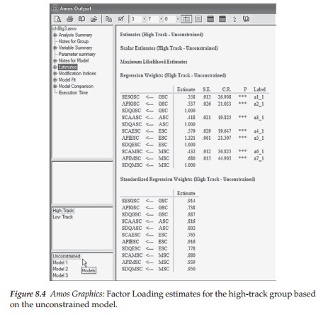
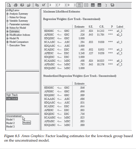
To familiarize you with the Amos output directory tree in multigroup analyses, I include here both the unstandardized and standardized factor loading estimates for the configural model. Figure 8.4 is pertinent to the high-track group, while Figure 8.5 is pertinent to the low-track group. In reviewing both of these figures, I direct your attention to four import­ant pieces of information. First, turning to the directory tree shown in the first section on the left side of Figure 8.4 you will note below that “High Track” is highlighted, thereby indicating that all results presented in this output file pertain only to this group. In contrast, if you were to click on “Low Track,” results pertinent to that group would be pre­sented. Second, below this group identification section of the tree, you will see a list of four models (unconstrained + three constrained). As indicated by the cursor at the bottom of this section, results presented here (and in Figure 8.5) relate to the unconstrained model. Third, because there are no constraints specified in this model, the parameters are freely estimated and, thus, vary across high- and low-track students. Finally, although equality constraints were not assigned to the factor loadings, the program automatically assigned labels that can be used to identify both the parameters and the groups in subsequent tests for invariance. These labels appear in the last column of the unstandardized estimates related to the Regression weights. For example, the label assigned to the factor loading of SESGSC on GSC is a1_1 for high-track students and a1_2 for low-track students.³

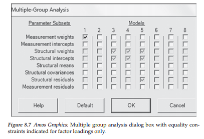
Testing for measurement invariance. Subsequent to the configural model, all tests for invariance require the imposition of equality constraints across groups. Implementation of this process, using the automated approach, begins with the hypothesized model open followed by selection of the Multiple-Group Analysis tab from the Analysis drop-down menu as illus­trated in the previous chapter (Figure 7.13). Clicking on this selection will present you with the warning message shown overlapping the Amos Graphics-labeled configural model in Figure 8.6. However, once you click on the OK button, you will immediately be presented with the Multiple-Group Analysis dialog box in which the first five columns show default parameter subsets that are checked. Some of the boxed checkmarks will be in bolded print, while others will appear faded, indicating that they are inactive, but cannot manually be deleted. In particular, the latter marks appear in columns 3 to 5 and represent structural weights, structural intercepts, and structural residuals, respectively, which are default parameters pertinent to full SEM models only. As I emphasized in Chapter 7, in testing for the invariance of all models, I consider it prudent to test first for invariance related to only the factor loadings. In this way, should the results yield evidence of noninvariance, you can then conduct follow-up analyses to determine which factor loading parameters are not operating the same way across groups and can exclude them from further analyses. Thus, in testing for invariance related only to the factor loadings, you will need to delete all bolded checkmarks from the Multiple-Group Analysis dialog box, except for the one in Column 1 (see Figure 8.7) representing only the “measurement weights.”

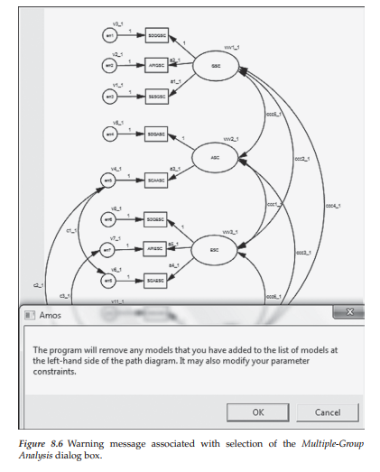
Once you click on the OK button of this dialog box, you will then see the assignment of constraint labels to your model. As shown in Figure 8.3, our hypothesized multigroup model with the appropriate factor loading estimates labeled (a2_2 to a6_2), in addition to those representing the fac­tor variances (vvv1_2 to vvv4_2), factor covariances (ccc1_2 to ccc6_2), and error variances (v1_2 to v11_2) as they pertain to Group 2, the low-track group. Likewise, labeling for the high-track (Group 1), is retrieved by clicking on the related group tab in the Amos output directory tree. As such the labeling system uses the number “1” to indicate its relevance to this group of students (e.g., a2_1; a3_1).

Goodness-of-fit results from this test of invariant factor loadings again provided evidence of a well-fitting model (x²(₇₇) = 245.571; CFI = .972; RMSEA = .052). Although the difference in x² from the configural model was statically significant (Ax²_w = 20.273), the difference between the CFI values met the recommended cutoff criterion of .01 (ACFI = .003). Using the CFI difference test as the criterion upon which to determine evidence of invariance, I concluded the factor loadings to be operating similarly across high-track and low-track students.

Testing for latent mean differences. As noted earlier, in testing for differ­ences in latent factor means, it is necessary to constrain both the factor load­ings and the observed variable intercepts equal across the groups. Consistent with the case for factor loadings, given findings of noninvariance pertinent to the intercepts, it becomes necessary to then conduct additional analyses to determine exactly which intercept or combination of intercepts is con­tributing to the inequality of intercepts across groups. As with the factor loadings, implementation of partial measurement invariance can be used provided that there is more than one invariant intercept over and above the reference variable (fixed to 1.00) for each latent factor (see Byrne et al., 1989; Muthen & Muthen, 1998-2012, p. 486). Admittedly, there has been, and still is much debate (see Chapter 7) and confusion concerning the issue of par­tial measurement invariance, particularly as it applies to the intercepts in the ultimate task of testing for latent mean differences. However, clearly it makes little sense to maintain equality constraints on intercepts that are not, in fact, operating equivalently across the groups under test.

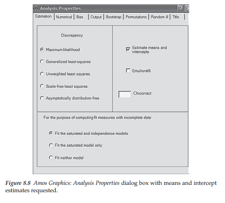
Our first step in testing for latent mean differences, then, is to con­strain the intercepts equal across groups. This task is easily accomplished by activating the Analysis Properties dialog box, either by clicking on its related icon or by selecting it from the Analysis drop-down menu. Once the Analysis Properties dialog box is open, we click on the Estimation tab and then select the Estimate means and intercepts option as shown in Figure 8.8.

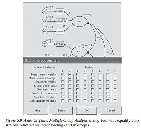
The next step in the process is to once again select the Multiple-Group Analysis option from the Analysis drop-down menu. This time, however, in addition to placing a checkmark in Column 1 for only the measure­ment weights, we additionally check off Column 2, which incorporates both the measurement weights and the measurement intercepts. Once these choices have been initiated, Amos automatically assigns a zero fol­lowed by a comma (0,) to each factor. Figure 8.9 captures this labeling action by showing both the options checked in the Multiple-Group Analysis dialog box, together with the resulting assignment of “0,” to the General SC (GSC) and Academic SC (ASC) factors.

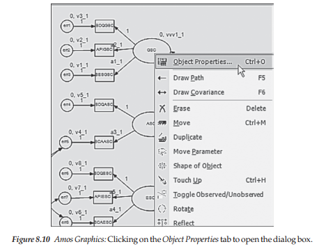
The fixed zero values shown in Figure 8.9 are assigned to the model relevant to each group. However, as discussed at the beginning of this chapter, in testing for latent mean differences, one of the groups is freely estimated while the other is constrained equal to some fixed amount. In the case here, Amos automatically fixes this zero value for both groups. Thus, the next step in the process is to remove these fixed factor values for one of the groups. The decision of which group will be fixed to zero is an arbitrary one and has no bearing on the final estimated mean values; regardless of which group is chosen, the results will be identical. In the present case, I elected to use the low-track group as the reference group (i.e., the latent means were fixed to a value of 0.0) and thus, moved on to removing the mean constraints for the high-track group. With the model open, this process begins by first highlighting the factor to be re-labeled by means of a left click of the mouse and then right-clicking on this factor, which will activate the Object Properties tab as shown in Figure 8.10.

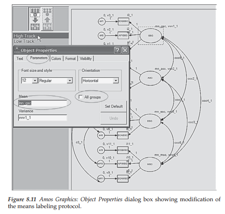
Clicking on this tab opens the Object Properties dialog box, after which we click on the Parameters tab; this action enables the re-labeling of the mean parameters. Our interest here is in removing the fixed zero value assigned to each of the factor means and replacing them with a label that allows these parameters to be freely estimated for the high-track group; Figure 8.11 captures this process. More specifically, when the dialog box was first opened, the label seen in the space below “mean” was 0. I sub­sequently replaced this number with an appropriate label (e.g., mn_gsc) that could be modified in accordance with its related factor as can be seen on the model behind. Circled within the dialog box, you can see assign­ment of the label to be assigned to the first factor (GSC). Note also, that the square beside “All groups” is empty and remains empty as we do not wish these re-labeling changes to be applied to both groups.⁴

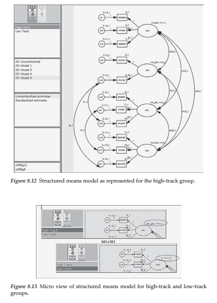
The final model to be tested for latent mean differences is shown in Figure 8.12 as it relates to the high-track group. However, clicking on the low-track label in the directory tree presents the same model, albeit with the zero values assigned to each of the factors. A mini version of both models is displayed in Figure 8.13.

Selected Amos Output: Model Summary

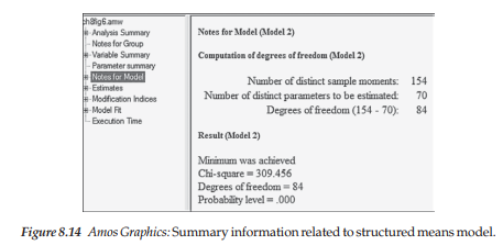
Of primary interest in analyses related to structured means models are (a) the latent mean estimates, and (b) the goodness-of-fit between the hypothesized model and the multigroup data. Before turning to these results for our analysis of high and low-track students, let’s once again take a few minutes to review a summary of the model in terms of the number of estimated parameters and resulting degrees of freedom. This summary is presented in Figure 8.14.

As you know by now, in order to calculate the degrees of freedom associated with the test of a model, you need to know two pieces of infor­mation: (a) the number of sample moments, and (b) the number of esti­mated parameters. In Figure 8.14, we see that there are 154 distinct sample moments and 70 estimated parameters. Let’s turn first to the number of sample moments. If you had calculated the number of moments in the same manner used with all other applications in this book, you would arrive at the number “132” ([11 x 12)/2] = 66; given two groups, the total is 132). Why this discrepancy? The answer lies in the analysis of covariance versus mean structures. All applications prior to the present chapter were based on covariance structures and, thus, the only pieces of information needed for the analyses were the covariances among the observed vari­ables. However, in the analysis of structured means models, information related to both the covariance matrix and the sample means is required which, as noted earlier, constitutes the moment matrix. With 11 observed variables in the model, there will be 11 means; 22 means for the two groups. The resulting number of moments, then, is 132 + 22 = 154.

Turning next to the reported 70 estimated parameters, let’s look first at the number of parameters being estimated for the high-track group.

As such, we have: 7 factor loadings, 9 covariances (6 factor covariances; 3 error covariances), 15 variances (11 error variances; 4 factor variances), 11 intercepts, and 4 latent means, yielding a total of 46 parameters to be estimated. For the low-track group, on the other hand, we have: only 9 covariances and 15 variances, resulting in a total of 24 parameters to be estimated; the factor loadings and intercepts have been constrained equal to those of the high-track group, and the latent means have been fixed to 0.0. Across the two groups, then, there are 70 (46 + 24) parameters to be estimated. With 154 sample moments, and 70 estimated parameters, the number of degrees of freedom will be 84.⁵

Selected Amos Output: Goodness-of-fit Statistics

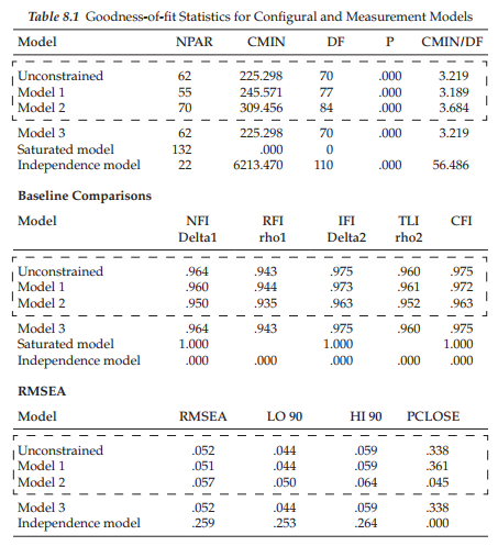
To provide you with a basis of comparison between the structured means model (Model 2 in the output) and both the configural model (i.e.,unconstrained model) and measurement model in which only the factor loadings were group invariant (Model 1 in the output), goodness-of-fit sta­tistics related to each are reported in Table 8.1. In each case, the fit statistics indicated well-fitting models. As reported earlier, although comparisons of Model 1 and 2 with the unconstrained model results in x²-difference tests that were statistically significant (p < .01 and p < .001, respectively), the CFI-difference tests met the Cheung and Rensvold (2002) cutoff cri­teria of <.01 (with rounding in the case of Model 2). Indeed, despite the equality constraints imposed on both the factor loadings and the observed variable intercepts across the two groups, the structured means model fitted the data exceptionally well (e.g., CFI = .963) and demonstrated an adequate approximation to the two adolescent ability track populations (RMSEA = .057). Given these findings, then, we can feel confident in inter­preting the estimates associated with the current solution.

Selected Amos Output: Parameter Estimates

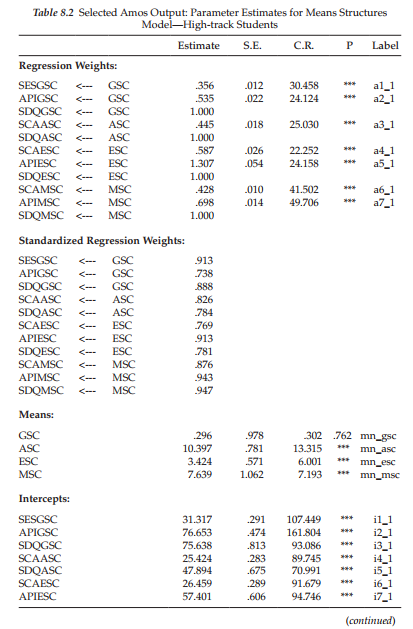
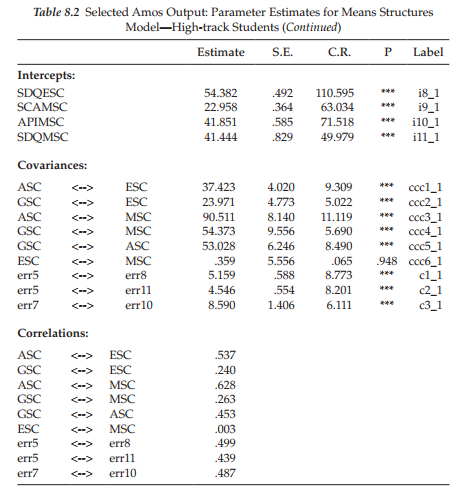
High-track students. We turn first to parameter estimates for the high-track group, which are reported in Table 8.2. In the interest of space, factor and error variances are not included. A brief perusal of the critical ratios (C.R.s) associated with these estimates reveals all, except the covariance between the factors ESC and MSC, to be statistically significant. This nonsignificant finding, however, is quite consistent with self-concept theory as it relates to these two academic dimensions and therefore is no cause for concern.

Of major interest here are the latent mean estimates reported for high-track students as they provide the key to the question of whether the latent factor means for this group are significantly different from those for low-track students. Given that the low-track group was designated as the reference group and thus their factor means were fixed to zero, the values reported here represent latent mean differences between the two groups. Reviewing these values we see that whereas the latent factor means related to the more specific facets of academic, English, and mathematics self-concepts were statistically significant (as indicated by the critical ratio values >1.96), this was not the case for general self-concept (C.R.=.304).

Given that the latent mean parameters were estimated for the high-track group, and that they represent positive values, we interpret these findings as indicating that, on average, high-track students in secondary school appear to have significantly higher perceptions of self than their low-track peers with respect to perceived mathematics and English capabilities, as well as to overall academic achievement in general. On the other hand, when it comes to a global perception of self, there appears to be little difference between the two groups of students. Readers interested in a more detailed discussion of these results from a substantive perspective are referred to the original article (Byrne, 1988b). The rationale for this interpretation derives from the fact that the observed variable intercepts were constrained equal across groups and thus, the latent factors have an arbitrary origin (i.e., mean). As a consequence, the latent factor means are not estimated in an absolute sense, but rather, reflect average differences in the level of self-perceptions across these two groups (see Brown, 2006).

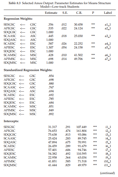
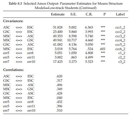
Low-track students. Turning now to the results for low-track students reported in Table 8.3, we find that, consistent with the high-track group, all parameter estimates are statistically significant except for the factor covariance between English and Math SC. Upon further scrutiny, how­ever, you may think that something is amiss with this table as both the factor loadings (i.e., regression weights) and the observed variable inter­cepts, as well as their related labels are identical to those reported for the high-track group. These results are correct, of course, as these parameters (for the low-track group) were constrained equal to those estimated for the high-track group. Finally, it is important to note that no estimates for the factor means are reported. Although these values were constrained to zero, Amos does not report these fixed values in the output.

In the example application illustrated in this chapter, model compari­sons based on CFI-difference values <.01 (Cheung & Rensvold, 2002) were used in determining measurement invariance of both the factor loadings and observed variable intercepts. However, if these model comparisons had resulted in CFI-difference values that had exceeded the cutpoint of .01, it would have been necessary to determine which individual factor loadings and/or intercepts were noninvariant. This process was demon­strated in Chapter 7 with respect to factor loadings; the same approach is used for the intercepts. In walking you through both the manual and auto­mated approaches to tests for invariance in Chapter 7 and 8, respectively, I hope that I have succeeded in helping you to feel sufficiently comfortable and confident in using either approach in analyses of your own data.

Source: Byrne Barbara M. (2016), Structural Equation Modeling with Amos: Basic Concepts, Applications, and Programming, Routledge; 3rd edition.