Application 4: Testing the Validity of a Causal Structure with AMOS

1. Key Concepts

• The full structural equation model
• Issue of item parceling
• Addressing evidence of multicollinearity
• Parameter change statistic
• Issue of model parsimony and nonsignificant parameter estimates
• Calculation and usefulness of the squared multiple correlation

In this chapter, we take our first look at a full structural equation model (SEM). The hypothesis to be tested relates to the pattern of causal structure linking several stressor variables that bear on the construct of teacher burnout. The original study from which this application is taken (Byrne, 1994b) tested and cross-validated the impact of organiza­tional (role ambiguity, role conflict, work overload, classroom climate, decision-making, superior support, peer support) and personality (self-esteem, external locus of control) variables on three dimensions of burnout (emotional exhaustion, depersonalization, reduced personal accomplishment) for elementary (N = 1,203), intermediate (N = 410), and secondary (N = 1,431) teachers. For each teaching panel, the data were subsequently randomly split into two (calibration and validation groups) for purposes of cross-validation. The hypothesized model of causal structure was then tested and cross-validated for elementary, intermediate, and secondary teachers. The final best-fitting and most parsimonious model was subsequently tested for the equivalence of causal paths across the three panels of teachers. For purposes of illus­tration in this chapter, we focus on testing the hypothesized causal structure based on the calibration sample of elementary teachers only (N = 599).

As was the case with the factor analytic applications illustrated in Chapters 3 through 5, full SEM models are also of a confirmatory nature. That is to say, postulated causal relations among all variables in the hypothesized model must be grounded in theory and/or empirical research. Typically, the hypothesis to be tested argues for the validity of specified causal linkages among the variables of interest. Let’s turn now to an in-depth examination of the hypothesized model under study in the current chapter.

2. The Hypothesized Model

The original intent of the 1994 paper cited here was to develop and test a model that described the nomological within- and between-network of variables (see Cronbach & Meehl, 1955) associated with burnout consist­ent with theory. However, much to my surprise, I discovered that at that time, in the early 1990s, there simply was no theory of burnout in gen­eral, or of teacher burnout in particular. In addition, to the best of my knowledge at that time, there was no solidly known array of variables that could be regarded as determinants of teacher burnout. Thus, it seemed apparent that the only way forward in gleaning this information was to review the literature pertinent to all research that had sought to identify factors contributing to teacher burnout. Most, but not all of these studies were based on multiple regression analyses. Formulation of the hypoth­esized model shown in Figure 6.1, derived from the consensus of findings from this review of the burnout literature as it bore on the teaching pro­fession. (Readers wishing a more detailed summary of this research are referred to Byrne, 1994b, 1999).

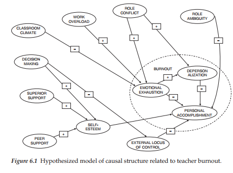
In reviewing this model, you will note that burnout is represented as a multidimensional construct with Emotional Exhaustion (EE), Depersonalization (DP), and Personal Accomplishment (PA) operating as conceptually distinct factors. This part of the model is based on the work of Leiter (1991) in conceptualizing burnout as a cognitive-emotional reac­tion to chronic stress. The paradigm argues that EE holds the central pos­ition because it is considered to be the most responsive of the three facets to various stressors in the teacher’s work environment. Depersonalization and reduced PA, on the other hand, represent the cognitive aspects of burnout in that they are indicative of the extent to which teachers’ per­ceptions of their students, their colleagues, and they themselves become diminished. As indicated by the signs associated with each path in the model, EE is hypothesized to impact positively on DP, but negatively on PA; DP is hypothesized to impact negatively on PA.

The paths (and their associated signs) leading from the organiza­tional (role ambiguity, role conflict, work overload, classroom climate, decision-making, superior support, peer support) and personality (self-esteem, external locus of control) variables to the three dimensions of burnout reflect findings in the literature.¹ For example, high levels of role conflict are expected to cause high levels of emotional exhaustion; in con­trast, high (i.e., good) levels of classroom climate are expected to generate low levels of emotional exhaustion.

3. Modeling with Amos Graphics

In viewing the model shown in Figure 6.1 we see that it represents only the structural portion of the full SEM (or equivalently, latent variable model). Thus, before being able to test this model, we need to know the manner by which each of the constructs in this model is measured. In other words, we now need to specify the measurement portion of the model (see Chapter 1). In contrast to the CFA models studied previously, the task involved in devel­oping the measurement model of a full SEM in this particular example² is twofold: (a) to determine the number of indicators to use in measuring each construct, and (b) to identify which items to use in formulating each indicator.

Formulation of Indicator Variables

In the applications examined in Chapters 3 through 5, the formulation of measurement indicators has been relatively straightforward; all examples have involved CFA models and, as such, comprised only measurement models. In the measurement of multidimensional facets of self-concept (see Chapter 3), each indicator represented a subscale score (i.e., the sum of all items designed to measure a particular self-concept facet). In

Chapters 4 and 5, our interest focused on the factorial validity of a meas­uring instrument. As such, we were concerned with the extent to which items loaded onto their targeted factor. Adequate assessment of this speci­fication demanded that each item be included in the model. Thus, the indi­cator variables in these cases each represented one item in the measuring instrument under study.

In contrast to these previous examples, formulation of the indicator variables in the present application is slightly more complex. Specifically, multiple indicators of each construct were formulated through the judi­cious combination of particular items to comprise item parcels. As such, items were carefully grouped according to content in order to equalize the measurement weighting across the set of indicators measuring the same construct (Hagtvet & Nasser, 2004). For example, the Classroom Environment Scale (Bacharach, Bauer, & Conley (1986), used to measure Classroom Climate, consists of items that tap classroom size, ability/inter- est of students, and various types of abuse by students. Indicators of this construct were formed such that each item in the composite measured a different aspect of classroom climate. In the measurement of classroom climate, self-esteem, and external locus of control, indicator variables con­sisted of items from a single unidimensional scale; all other indicators com­prised items from subscales of multidimensional scales. This meaningful approach to parceling is termed purposive parceling, as opposed to random (or quasi) parceling, which Bandalos and Finney (2001) found to be the most commonly used form of parceling. (For an extensive description of the measuring instruments, see Byrne, 1994b.) In total, 32 item-parcel indi­cator variables were used to measure the hypothesized structural model.

In the period since the study examined here was conducted, there has been a growing interest in the viability of item parceling. Research con­cerns have focused on such issues as methods of item allocation to parcels (Bandalos & Finney, 2001; Hagtvet & Nasser, 2004; Kim & Hagtvet, 2003; Kishton & Widaman, 1994; Little, Cunningham, Shahar, & Widaman, 2002; Rogers & Schmitt, 2004; Sterba & MacCallum, 2010), number of items to include in a parcel (Marsh, Hau, Balla, & Grayson, 1998), extent to which item parcels affect model fit (Bandalos, 2002), and, more generally, whether or not researchers should even engage in item parceling at all (Little et al., 2002; Little, Lindenberger, & Nesselroade, 1999; Little, Rhemtulla, Gibson, & Schoemann, 2013; Marsh, Ludke, Nagengast, Morin, & Von Davier, 2013). Little et al.(2002) present an excellent summary of the pros and cons of using item parceling; the Bandalos and Finney (2001) chapter gives a thorough review of the issues related to item parceling; and the Marsh et al. (2013) paper offers a substantial historical perspective on the use of parceling. (For details related to each of these aspects of item parceling, readers are advised to consult these references directly.)

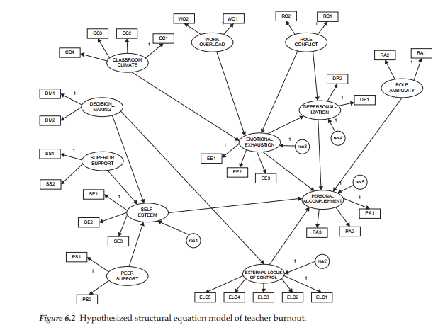
A schematic presentation of the hypothesized full SEM model is pre­sented in Figure 6.2. It is important to note that, in the interest of clarity and space restrictions, all double-headed arrows representing correla­tions among the independent (i.e., exogenous) factors, in addition to the measurement error associated with each indicator variable, have been excluded from the figure. However, given that Amos Graphics operates on the WYSIWYG (what you see is what you get) principle, these parameters must be included in the model before the program will perform the ana­lyses. I revisit this issue after we fully establish the hypothesized model under test in this chapter.

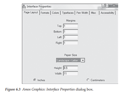
The preliminary model (because we have not yet tested for the val­idity of the measurement model) in Figure 6.2 is most appropriately pre­sented within the framework of the landscape layout. In Amos Graphics, this is accomplished by pulling down the View menu and selecting the Interface Properties dialog box, as shown in Figure 6.3. Here you see the open Page Layout tab that enables you to opt for Landscape orientation.

Confirmatory Factor Analyses

Because (a) the structural portion of a full structural equation model involves relations among only latent variables, and (b) the primary con­cern in working with a full SEM model is to assess the extent to which these relations are valid, it is critical that the measurement of each latent variable be psychometrically sound. Thus, an important preliminary step in the analysis of full SEM models is to test first for the validity of the measurement model before making any attempt to evaluate the structural model. Accordingly, CFA procedures are used in testing the validity of the indicator variables. Once it is known that the measurement model is oper­ating adequately,³ one can then have more confidence in findings related to the assessment of the hypothesized structural model.

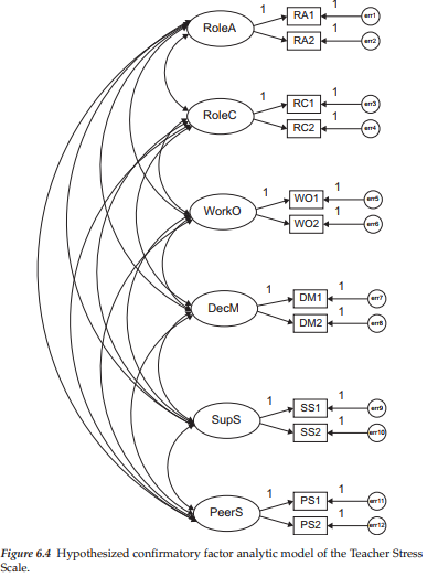
In the present case, CFAs were conducted for indicator variables derived from each of the two multidimensional scales; these were the Teacher Stress Scale (TSS; Pettegrew & Wolf, 1982), which included all organizational indicator variables except classroom climate, and the Maslach Burnout Inventory (MBI; Maslach & Jackson, 1986), measuring the three facets of burnout. The hypothesized CFA model of the TSS is portrayed in Figure 6.4.

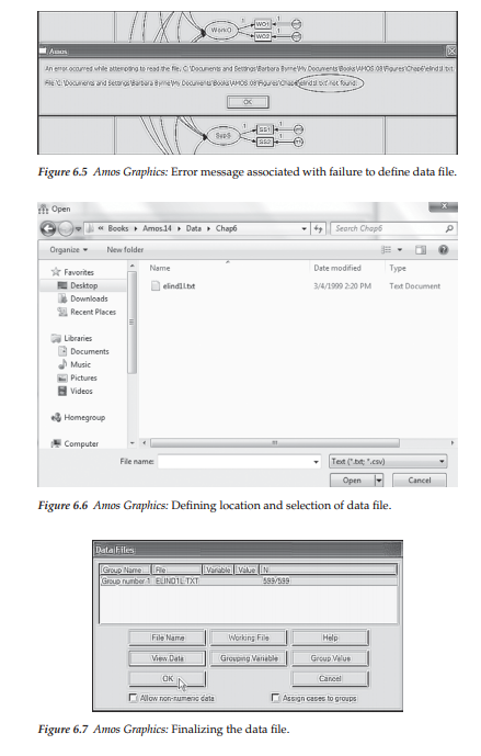
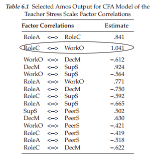
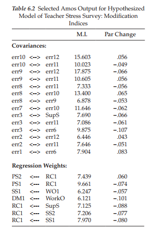
Of particular note here is the presence of double-headed arrows among all six factors. Recall from Chapter 2 and earlier in this chapter, that Amos Graphics assumes no correlations among the factors. Thus, should you wish to estimate these values in accordance with the related theory, they must be present in the model. However, rest assured that the program will definitely prompt you should you neglect to include one or more factor correlations in the model. Another error message that you are bound to receive at some time prompts that you forgot to identify the data file upon which the analyses are to be based. For example, Figure 6.5 presents the error message triggered by my failure to establish the data file a priori. However, this problem is quickly resolved by clicking on the Data icon (H; or select Data Files from the File dropdown menu), which then triggers the dialog box shown in Figure 6.6. Here you simply locate and click on the data file, and then click on Open). This action subsequently produces the Data Files dialog box shown in Figure 6.7, where you will need to click on OK.

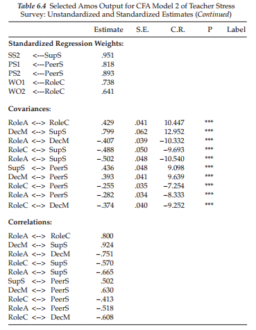
Although goodness-of-fit for both the MBI (CFI = .98) and TSS (CFI = .973) were found to be exceptionally good, the solution for the TSS was somewhat problematic. More specifically, a review of the standard­ized estimates revealed a correlation value of 1.041 between the factors of Role Conflict and Work Overload, a warning signal of possible multicol- linearity; these standardized estimates are presented in Table 6.1.

Multicollinearity arises from the situation where two or more variables are so highly correlated that they both, essentially, represent the same under­lying construct. Substantively, this finding is not surprising as there appears to be substantial content overlap among the TSS items measuring role con­flict and work overload. The very presence of a correlation >1.00 is indicative of a solution that is clearly inadmissible. Of course, the flip side of the coin regarding inadmissible solutions is that they alert the researcher to serious model misspecifications. However, a review of the modification indices (see Table 6.2) provided no help whatsoever in this regard. All Parameter Change statistics related to the error covariances revealed nonsignificant values less than or close to 0.1 and all MIs for the regression weights (or factor loadings) were less than 10.00, again showing little to be gained by specifying any cross-loadings. In light of the excellent fit of Model 2 of the TSS, together with these nonthreatening MIs, I see no rational need to incorporate addi­tional parameters into the model. Thus, it seemed apparent that another tac­tic was needed in addressing this multicollinearity issue.

One approach that can be taken in such instances is to combine the measures as indicators of only one of the two factors involved. In the present case, a second CFA model of the TSS was specified in which the factor of Work Overload was deleted, albeit its two observed indicator variables were loaded onto the Role Conflict factor. Goodness-of-fit related to this 5-factor model of the TSS (x² ₍₄₄₎ = 152.374; CFI = .973; RMSEA = .064) exhibited an exceptionally good fit to the data. The model summary and parameter esti­mates related to both the unstandardized and standardized factor loadings and factor covariances are shown in Tables 6.3 and 6.4, respectively.

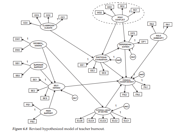
This 5-factor structure served as the measurement model for the TSS throughout analyses related to the full causal model. However, as a consequence of this measurement restructuring, the revised model of burnout shown in Figure 6.8 replaced the originally hypothesized model (see Figure 6.2) in serving as the hypothesized model to be tested. Once again, in the interest of clarity, the factor correlations and measurement errors are not included in this diagram.

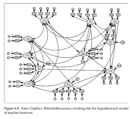
At the beginning of this chapter, I mentioned that Amos Graphics operates on the WYSIWYG principle and therefore, unless factor covari­ances and error terms are specified in the model, they will not be esti­mated. I promised to revisit this issue and I do so here. In the case of full SEM models, for failure to include double-headed arrows among the exogenous factors, as in Figure 6.8 (Role Ambiguity, Role Conflict, Classroom Climate, Decision-making, Superior Support, Peer Support), as well as the error variances and their related regression paths, Amos will prompt you with a related error message. However, there is really no way of adding these parameters to the existing model in a neat and clear manner. Rather, the model becomes very messy-looking, as dis­played in Figure 6.9. It is for this reason that I did not include these parameters in Figure 6.8.

Selected Amos Output: Hypothesized Model

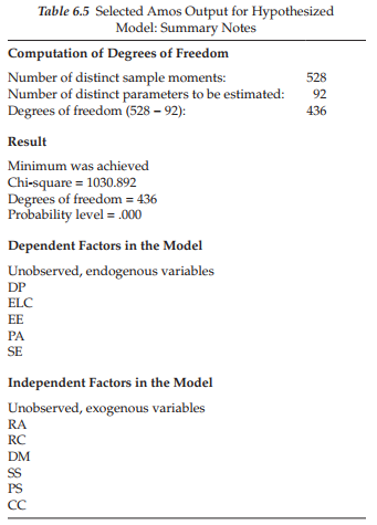
Before examining test results for the hypothesized model, it is instructive to first review summary notes pertinent to this model, which are presented in four sections in Table 6.5. The initial information advises that (a) the anal­yses are based on 528 sample moments (32 [indicator measures] x 33/2), (b) there are 92 parameters to be estimated, and (c) by subtraction, there are 436 degrees of freedom. The next section reports on the bottom-line information that the minimum was achieved in reaching a convergent solution and yielding a x² value of 1,030.892 with 436 degrees of freedom.

Summarized in the lower part of the table are the dependent and independent factors in the model. Specifically, there are five dependent (or endogenous) factors in the model (DP; ELC; EE; PA; SE). Each of these factors has single-headed arrows pointing at it, thereby easily identifying it as a dependent factor in the model. The independent (or exogenous) factors are those hypothesized as exerting an influence on the dependent factors; these are RA, RC, DM, SS, PS, and CC.

Model Assessment

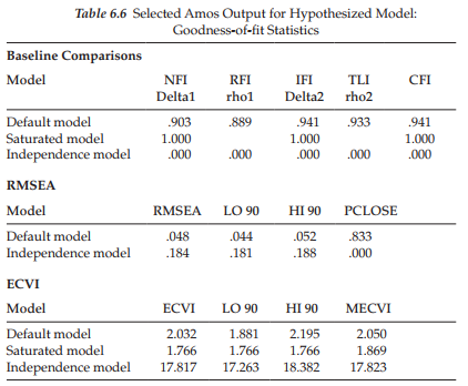
Goodness-of-fit summary. Selected oodness-of-fit statistics related to the hypothesized model are presented in Table 6.6. In Table 6.5, we observed that the overall x² value, with 436 degrees of freedom, is 1,030.892. Given the known sensitivity of this statistic to sample size, however, use of the x² index provides little guidance in determining the extent to which  the model does not fit. Thus, it is more reasonable and appropriate to base decisions on other indices of fit. Primary among these are the CFI, RMSEA, and standardized RMR (SRMR). As noted in Chapter 3, the SRMR is not included in the output, and must be calculated separately. In addition, given that we shall be comparing a series of models in our quest to obtain a final well-fitting model, the ECVI is also of interest.

is used within a relative framework. (For a review of these rule-of-thumb guidelines, you may wish to consult Chapter 3 where goodness-of-fit indi­ces are described in more detail.)

Modification indices. Over and above the fit of the model as a whole, however, a review of the modification indices reveals some evidence of misfit in the model. Because we are interested solely in the causal paths of the model at this point, only a subset of indices related to the regression weights is included in Table 6.7. Turning to this table, you will note that the first 10 modification indices (MIs) are enclosed in a rectangle. These parameters represent the structural (i.e., causal) paths in the model and are the only MIs of interest. The reason for this statement is because in work­ing with full SEMs, any misfit to components of the measurement model should be addressed when that portion of the model is tested for its val­idity. Some of the remaining MIs in Table 6.7 represent the cross-loading of an indicator variable onto a factor other than the one it was designed to measure (EE3 ^ CC). Others represent the regression of one indicator variable on another; these MIs are substantively meaningless.⁴

In reviewing the information encased within the rectangle, we note that the maximum MI is associated with the regression path flowing from Classroom Climate to Depersonalization (DP <— CC). The value of 24.776 indicates that, if this parameter were to be freely estimated in a subse­quent model, the overall x² value would drop by at least this amount. If you turn now to the Parameter Change statistic related to this parameter, you will find a value of -0.351; this value represents the approximate value that the newly estimated parameter would assume. I draw your attention also to the four highlighted regression path MIs. The common link among these parameters is that the direction of the path runs coun­ter to the general notion of the postulated causal model. That is, given that the primary focus is to identify determinants of teacher burnout, the flow of interest is from left to right. Although admittedly there may be some legitimate reciprocal paths, they are not of substantive interest in the present study.

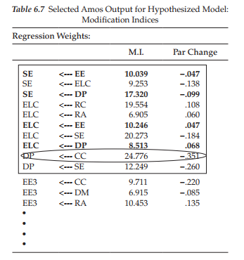
In data preparation, the TSS items measuring Classroom Climate were reflected such that low scores were indicative of a poor classroom milieu, and high scores, of a good classroom milieu. Turning now to the MI of interest here, it would seem perfectly reasonable that elementary school teachers whose responses yielded low scores for Classroom Climate, should concomitantly display high levels of depersonalization. Given the meaningfulness of this influential flow, then, the model was reestimated with the path from Classroom Climate to Depersonalization specified as a freely estimated parameter; this model is subsequently labeled as Model 2. Results related to this respecified model are subsequently discussed within the framework of post hoc analyses.

Post Hoc Analyses

Selected Amos Output: Model 2

In the interest of space, only the final model of burnout, as determined from the following post hoc model-fitting procedures, will be displayed. However, relevant portions of the Amos output, pertinent to each respeci­fied model, will be presented and discussed.

Model Assessment

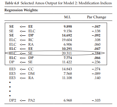
Goodness-of-fit summary. The estimation of Model 2 yielded an over­all x²(₄₃₅) value of 995.019, a CFI of .945, an SRMR value of .058, and a RMSEA of .046; the ECVI value was 1.975. Although the improvement in model fit for Model 2, compared with the originally hypothesized model, would appear to be trivial on the basis of the CFI, and RMSEA values, the model difference nonetheless was statistically significant (Ax²(1) = 35.873). Moreover, the parameter estimate for the path from Classroom Climate to Depersonalization was slightly higher than the one predicted by the Expected Parameter Change statistic (-0.479 versus -0.351) and it was statistically significant (C.R. = -5.712). Modification indices related to the structural parameters for Model 2 are shown in Table 6.8.

Modification indices. In reviewing the boxed statistics presented in Table 6.8, we see that there are still nine MIs that can be taken into account in the determination of a well-fitting model of burnout, albeit four of these (highlighted and discussed earlier) are not considered in light of their reverse order of causal impact. The largest of these qualifying MIs (MI = 20.311) is associated with a path flowing from Self-esteem to External Locus of Control (ELC <— SE), and the expected value is estimated to be -.184. Substantively, this path again makes good sense as it seems likely that teachers who exhibit high levels of self-esteem are likely to exhibit low levels of external locus of control. On the basis of this rationale, we again focus on the path associated with the largest MI. Accordingly, the causal structure was again respecified—this time, with the path from Self-esteem to External Locus of Control freely estimated (Model 3).

Selected Amos Output: Model 3 Model Assessment

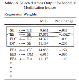
Goodness-of-fit summary. Model 3 yielded an overall x²(434) value of 967.244, with CFI = .947, SRMR = .053, and RMSEA = .045; the ECVI was 1.932. Again, the x²-difference between Models 2 and 3 was statistically signifi­cant (Ax²(₁) = 27.775). Modification indices related to Model 3 are shown in Table 6.9. Of initial import here is the fact that the number of MIs has now dropped from nine to only four, with only one of the original four reverse-order causal links now highlighted. This discrepancy in the num­ber of MI values between Model 2 and Model 3 serves as a perfect example of why the incorporation of additional parameters into the model must be done one at a time in programs that take a univariate approach to the assessment of MIs.

Modification indices. Reviewing the boxed statistics here, we see that the largest MI (17.074) is associated with a path from Self-esteem to Emotional Exhaustion (EE <— SE). However, it is important that you note that an MI (9.642) related to the reverse path involving these factors (SE <— EE) is also included as an MI. As emphasized in Chapter 3, parameters identified by Amos as belonging in a model are based on statistical criteria only; of more import, is the substantive meaningfulness of their inclusion. Within the context of the original study, the incorporation of this latter path (SE <—EE) into the model would make no sense whatsoever since its primary purpose was to validate the impact of organizational and person­ality variables on burnout, and not the reverse. Thus, again we ignore this suggested model modification.⁵ Because it seems reasonable that teachers who exhibit high levels of self-esteem may, concomitantly, exhibit low lev­els of emotional exhaustion, the model was reestimated once again, with the path, EE <— SE, freely estimated (Model 4).

Selected Amos Output: Model 4 Model Assessment

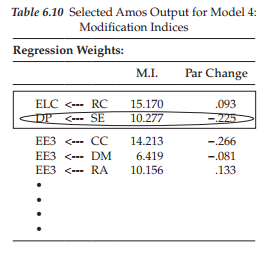
Goodness-of-fit summary. The estimation of Model 4 yielded a x² value of 943.243, with 433 degrees of freedom. Values related to the CFI, SRMR, and RMSEA were .949, .048, and .044, respectively; the ECVI value was 1.895. Again, the difference in fit between this model (Model 4) and its predeces­sor (Model 3) was statistically significant (Ax²(₁) = 24.001). Modification indices related to the estimation of Model 4 are presented in Table 6.10.

Modification indices. In reviewing these boxed statistics, note that the MI associated with the former regression path flowing from Emotional Exhaustion to Self-esteem (SE <— EE) is no longer present. We are left only with the paths leading from Role Conflict to External Locus of Control (ELC <— RC), and from Self-esteem to Depersonalization (DP <— SE). Although the former is the larger of the two (MI = 15.170 vs. 10.277), the latter exhibits the larger parameter change statistic (-.225 vs. .093). Indeed, some methodologists (e.g., Kaplan, 1989) have suggested that it may be more appropriate to base respecification on size of the parameter change statistic, rather than on the Ml (but recall Bentler’s [2005] caveat noted in Chapter 3, that these values can be affected by both the scaling and identification of factors and variables). Given that this parameter is substantively meaningful (i.e., high levels of SE should lead to low levels of DP, and vice versa), Model 4 was respecified to include the estimation of a regression path leading from Self-esteem to Depersonalization in a model now labeled Model 5.

Selected Amos Output: Model 5 Model Assessment

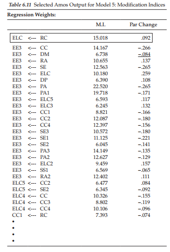
Goodness-of-fit summary. Results from the estimation of Model 5 yielded a x²(₄₃₂) value of 928.843, a CFI of .951, an SRMR of .047a, and an RMSEA of .044; the ECVI value was 1.874. Again, the improvement in model fit was found to be statistically significant (Ax²(₁) = 14.400. Finally, the esti­mated parameter value (-.315), which exceeded the parameter change statistic estimated value, was also statistically significant (C.R.= -.3.800). Modification indices related to this model are presented in Table 6.11.

Modification indices. Not unexpectedly, a review of the output related to Model 5 reveals an MI associated with the path from Role Conflict to External Locus of Control (ELC <— RC); note that the Expected Parameter Change statistic has remained minimally unchanged (.092 vs. .093). Once again, from a substantively meaningful perspective, we could expect that high levels of role conflict would generate high levels of external locus of control thereby yielding a positive Expected Parameter Change statistic value. Thus, Model 5 was respecified with the path (ELC <— RC) freely estimated, and labeled as Model 6.

Selected Amos Output: Model 6

Up to this point in the post hoc modeling process, we have focused on only the addition of parameters to the model. Given that all additional structural paths, as identified by the MIs, were found to be justified, we need now to examine the flip side of the coin – those originally specified structural paths that are shown to be redundant to the model. This issue of model parsimony is addressed in this section.

Model Assessment

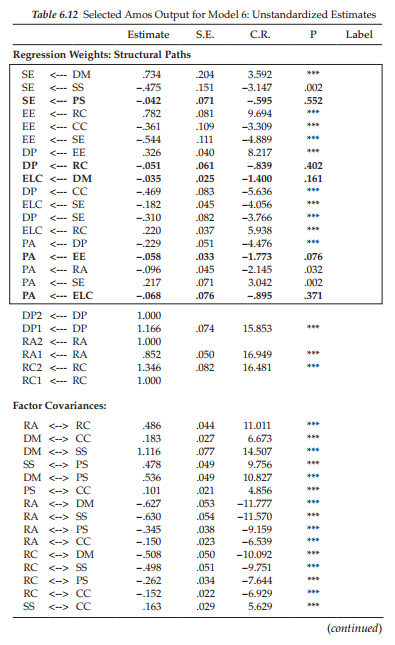
Goodness-of-fit summary. Estimation of Model 6 yielded an overall x²(₄₃₁) value of 890.619; again, the x²-difference between Models 5 and 6 was sta­tistically significant (Ax²^) = 38.224), as was the estimated parameter (.220, C.R. = 5.938), again much larger than the estimated parameter change statistic value of .092. Model fit statistics were as follows: CFI = .954, SRMR = .041, and RMSEA = .042; the ECVI dropped a little further to 1.814, thereby indicating that Model 6 represented the best fit to the data thus far in the analyses. As expected, no MIs associated with structural paths were present in the output; only MIs related to the regression weights of factor loadings remained. Thus, no further consideration was given to the inclu­sion of additional parameters. Unstandardized estimates related to Model 6 are presented in Table 6.12.

The Issue of Model Parsimony

Thus far, discussion related to model fit has focused solely on the addition of parameters to the model. However, another side to the question of fit, particularly as it pertains to a full model, is the extent to which certain initially hypothesized paths may be irrelevant to the model as evidenced from their statistical nonsignificance. In reviewing the structural param­eter estimates for Model 6, we see five parameters that are nonsignificant; these parameters represent the paths from Peer Support to Self-esteem (SE <— PS; C.R. = -.595; p = .552); Role Conflict to Depersonalization (DP <— RC; C.R. = -.839; p = .402); Decision-making to External Locus of Control (ELC <— DM; C.R. = -1.400; p = .161); Emotional Exhaustion to Personal Accomplishment (PA <— EE; C.R. = -1.773; p = .076); External Locus of Control to Personal Accomplishment (PA <— ELC; C.R. = -.895; p = .371). In the interest of parsimony, then, a final model of burnout needs to be estimated with these five structural paths deleted from the model. Importantly, as can be seen in Table 6.12, given that the factor of Peer Support (PS) neither has any influence on other factors nor is it influenced by other factors in the model, it no longer has any meaningful relevance and thus needs also to be eliminated from the model. Finally, before leaving Model 6, and Table 6.12, note that all factor variances and covariances are found to be statistically significant.

Because standardized estimates are typically of interest in presenting results from structural equation models, it is usually of interest to request these statistics when you have determined your final model. Given that Model 7 will serve as our final model representing the determinants of teacher burnout, this request was made by clicking on the Analysis Properties icon [M which, as demonstrated in Chapter 5, triggers the related dialog box and tabs. Select the Output tab and elect to have the standardized estimates included in the output file. In addition, it is also advisable to ask for the squared multiple correlations, an option made available on the same tab.

Selected Amos Output: Model 7 (Final Model)

As this revised model represents the final full SEM model to be tested in this chapter, several components of the Amos output file are presented and discussed. We begin by reviewing results related to the model assess­ment, which are displayed in Table 6.13.

Model Assessment

Goodness-of-fit summary. As shown in Table 6.13, estimation of this final model resulted in an overall x²(₃₈₂) value of 803.875. At this point, you may wonder why there is such a big difference in this x² value and its degrees of freedom compared with all previous models. The major reason, of course, is due to the deletion of one factor from the model (Peer Support).⁶ Relatedly, this deletion changed the number of sample moments, which in turn, substantially altered the number of degrees of freedom. To ensure that you completely understand how these large differences occurred, let’s just review this process as outlined earlier in the book.

The Peer Support factor had two indicator variables, PS1 and PS2. Thus, following its deletion, the number of observed measures dropped from 32 to 30. Based on the formula (p x [p + 1]/2) discussed earlier in the book, this reduction resulted in 30 x 31/2 (465) distinct sample moments (or elements in the covariance matrix). Given the estimation of 83 param­eters, the number of degrees of freedom is 382 (465 – 83). By comparison, had we retained the Peer Support factor, the number of sample moments would have been 32 x 33/2 (528). The number of estimated parameters would have increased by 9 (1 factor loading, 2 error variances, 1 factor variance, 5 factor covariances), resulting in a total of 92, and 436 (528 – 92) degrees of freedom. However, in the interest of scientific parsimony, as noted earlier, given its presence as an isolated factor having no linkages with other factors in the model, I consider it most appropriate to exclude the factor of Peer Support from the Model. Of import here is that this resulting change to the model now renders it no longer “nested” within the original model. As such, it would be inappropriate to calculate a chi-square difference value.

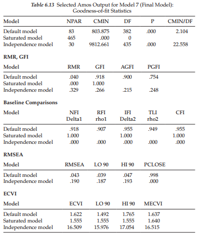
As evidenced from the remaining goodness-of-fit indices, this final model represented an excellent fit to the data (CFI = .955; SRMR = .041; RMSEA = .043). The ECVI value of 1.622 signals this final and most parsi­monious model to represent the best overall fit to the data. We turn next to an examination of the parameter estimates, which are presented in Table 6.14.

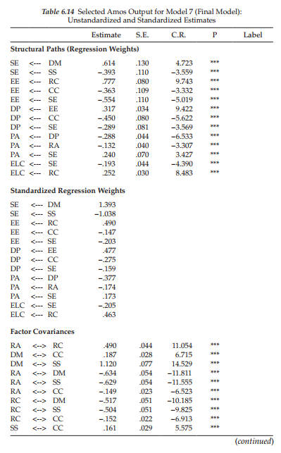
Parameter Estimates

Both the unstandardized and standardized estimates are presented in Table 6.14. However, in the interest of space, they are shown for only the structural paths and factor covariances; all factor and error variances (not shown), however, were found to be statistically significant. Turning first to the unstandardized estimates for the structural parameter paths, we see that all are statistically significant as indicated by the critical values and their related p-values. In a review of the standardized estimates, how­ever, there are two values that are somewhat worrisome given their values greater than 1.00; these represent the paths flowing from Decision-making to Self-esteem (SE <— DM) and from Superior Support to Self-esteem (SE <— SS). Although all remaining standardized estimates are sound, the two aberrant estimates signal the need for further investigation.

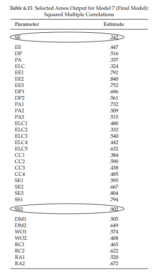
A review of the factor covariances again shows all to be statistically significant. However, in reviewing the standardized estimates, we again see a disturbingly high correlation between the factors of Decision-making and Superior Support (DM <—> SS), which clearly ties in with the exces­sively high estimates for the related factors noted in the previous section. Given these related atypical estimates, I consider it important to further probe the appropriateness of factors specified as determinants of teacher burnout. Before closing out this chapter, I return to this important and challenging issue, but first, let’s complete our review of this final model by turning to results for the squared multiple correlations (SMCs), which are reported in Table 6.15.

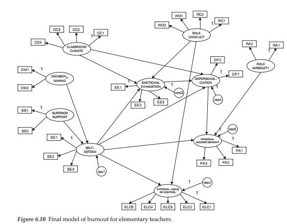
The SMC is a useful statistic that is independent of all units of meas­urement. Once it is requested, Amos provides an SMC value for each endogenous variable in the model. Thus, in Table 6.15, you will see SMC values for each dependent factor in the model (SE, EE, DP, PA, ELC) and for each of the factor loading regression paths (EE1-RA2). The SMC value represents the proportion of variance that is explained by the predictors of the variable in question. For example, in order to interpret the SMC associated with Self-esteem (SE; circled), we need first to review Figure 6.8 to ascertain which factors in the model serve as its predictors. Accordingly, we determine that 24.6% of the variance associated with Self-esteem is accounted for by its two predictors—Decision-making (DM) and Superior Support (SS), the factor of Peer Support (PS) having been subsequently deleted from the model. Likewise, we can determine that the factor of Superior Support explains 90.2% of the variance associ­ated with its second indicator variable (SS2; circled). The final version of this model of burnout for elementary teachers is schematically presented in Figure 6.10.

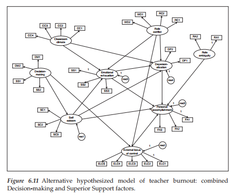
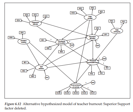
Let’s return now to the problematic estimates noted earlier with respect to structural paths leading from Decision-making (DM) and Superior Support (SS) to Self-esteem (SE), as well as the factor correla­tion between DM and SS. Clearly the difficulty arises from an overlap of content in the items measuring these three constructs. Aside from a thorough investigation of the items involved, another approach might be to specify and test two alternative models of teacher burnout. In the first model (Model A), combine the factors of DM and SS by loading the two SS indicator variables onto the DM factor, as we did in the case of Role Conflict and Work Overload. In the second model (Model B), delete the factor of SS completely from the model. A schematic presentation of Models A and B are presented in Figures 6.11 and 6.12, respectively. Importantly, I need once again to advise that these figures are shown minus the necessary factor correlation double arrows, as well as the error terms, all in the interest of clarity of presentation. However, as stressed earlier in this chapter, it is imperative that these parameters be added to the model prior to their analyses. Although restrictions of space prevent me from addressing these analyses here, you will definitely be reminded of this requirement through a pop-up error message. I strongly encour­age you to experiment yourself in testing these two alternative models using the same data that were used in testing the hypothesized model in this chapter, which can be found in the book’s companion website pro­vided by the publisher.

In working with structural equation models, it is very important to know when to stop fitting a model. Although there are no firm rules or regulations to guide this decision, the researcher’s best yardsticks include (a) a thorough knowledge of the substantive theory, (b) an adequate assessment of statistical criteria based on information pooled from vari­ous indices of fit, and (c) a watchful eye on parsimony. In this regard, the SEM researcher must walk a fine line between incorporating a suffi­cient number of parameters to yield a model that adequately represents the data, and falling prey to the temptation of incorporating too many parameters in a zealous attempt to attain the statistically best-fitting model. Two major problems with the latter tack are that (a) the model can comprise parameters that actually contribute only trivially to its structure, and (b) the more parameters there are in a model, the more difficult it is to replicate its structure should future validation research be conducted.

In bringing this chapter to a close, it may be instructive to sum­marize and review findings from the various models tested. First, of 13 causal paths specified in the revised hypothesized model (see Figure 6.8), eight were found to be statistically significant for elementary teachers. These paths reflected the impact of (a) classroom climate and role con­flict on emotional exhaustion, (b) decision-making and superior support on self-esteem, (c) self-esteem, role ambiguity, and depersonalization on perceived personal accomplishment, and (d) emotional exhaustion on depersonalization. Second, five paths, not specified a priori (Classroom Climate ^ Depersonalization; Self-esteem ^ External Locus of Control; Self-esteem ^ Emotional Exhaustion; Role Conflict ^ External Locus of

Control; Self-esteem ^ Depersonalization), proved to be essential com­ponents of the causal structure. Given their substantive meaningfulness, they were subsequently added to the model. Third, five hypothesized paths (Peer Support ^ Self-esteem; Role Conflict ^ Depersonalization; Decision-making ^ External Locus of Control; Emotional Exhaustion ^ Personal Accomplishment; External Locus of Control ^ Personal Accomplishment) were not statistically significant and were therefore deleted from the model. Finally, in light of the ineffectual impact of peer support on burnout for elementary teachers, this construct was also deleted from the model. In broad terms, based on our findings from this full SEM application, we can conclude that role ambiguity, role conflict, classroom climate, participation in the decision-making process, and the support of one’s superiors are potent organizational determinants of burnout for elementary school teachers. The process, however, appears to be strongly tempered by one’s sense of self-worth.

4. Modeling with Amos Tables View

Once again, I wish to give you at least a brief overview of the hypoth­esized model (Figure 6.8) as Amos displays it in Tables View format. Given the size of this full SEM model, however, it is very difficult, if not impossible, to clearly present all components within this framework. Nonetheless, I have tried my best to give you at least a miniature vision of the specification of the observed and latent variables, the regression paths, and the factor covariances. However, I need to point out that in build­ing in all covariances among the exogenous factors (Role Ambiguity, Role Conflict, Classroom Climate, Decision-making, Superior Support, and Peer Support), as well as all the error variances, limitations of space made it necessary to shorten the names of all latent factors in the model. Thus in reviewing this partial portrayal of the hypothesized model in Tables View format, you will see only 2- or 3-letter labels in lieu of the longer variable names as displayed in Figure 6.8. This partial Tables View format is shown in Figure 6.13.

As noted in Chapter 5, once again several of the entries for both the Variables and Regression weights entries are sometimes erratically placed in the listings such that there is not an orderly presentation of these specifi­cations. For example, in the Variables section on the left, you will see the entry for EE3 (the third indicator variable for Emotional Exhaustion [EE]) checked off as an observed variable, and its related error term (eee3), as a latent variable, which is therefore unchecked. However, EE2 and EE1, along with their error terms, are entered elsewhere in this first listing. Thus, when reviewing the Tables View format, I caution you to be careful in checking on the correctness of the specifications. As noted in Chapter 5, it is not possible to make any manual modification.

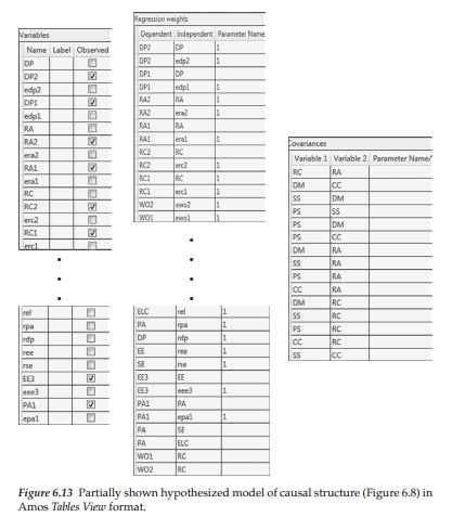
Turning to the Regression weights listing, let’s look at the first two entries for DP2, the second indicator variable for the factor of Depersonalization (DP). Although I had shown (and intended) DPI to serve as the referent variable for DP (i.e., its regression path to be fixed to 1.00), the imprecision of the Amos-drawn model led the program to interpret DP2 instead, as the referent indicator variable. Thus the first entry represents the regression of

DP2 onto the DP factor, but with the path fixed to 1.00. The second entry represents the regression path associated with the error variance for DP 2, which of course is fixed to 1.00. The third entry represents the regression of the first indicator variable for Depersonalization (DPI) as freely estimated and again, in the fourth entry, its related error term. Moving down to the entries in the lower part of this section, you will see the letter “r” preced­ing certain variables listed in the “Independent” column. For example, on the first entry of the lower list, we see ELC listed as the dependent variable and rel listed as the independent variable. This latter entry represents the residual associated with the dependent latent factor of External Locus of Control (ELC). All remaining entries shown in this Regression weights sec­tion are all interpretable in the same manner as explained with these three examples.

Finally, the third entry in this figure represents the Covariances speci­fied among all of the exogenous variables in the model. As noted earlier, the hypothesized model schematically displayed in Figure 6.8 is shown without these correlations and error terms for purposes of simplicity and clarity. However, it is important to emphasize that the model to be submit­ted for analysis by the program must include all of these parameters, other­wise you will receive related error messages. These additional parameters are easily added to the model but make for a very messy model as shown in Figure 6.9.

Unfortunately, given the length of the Tables View representation of models, I have been able only to show you bits and pieces of the entire output. However, it may be helpful in knowing that this formatted com­position of the model can simplify your check that all components are included in your model.

Source: Byrne Barbara M. (2016), Structural Equation Modeling with Amos: Basic Concepts, Applications, and Programming, Routledge; 3rd edition.