Application 9: Testing Change Over Time with AMOS: The Latent Growth Curve Model

1. Key Concepts

• Measuring change over three or more time points
• Intraindividual versus interindividual differences in change
• Factor intercept and slope as growth parameters
• Importance of the Amos plug-in menu
• Incorporating a time-invariant predictor of change
• Use of Amos Graphics interface properties option

Behavioral scientists have long been intrigued with the investigation of change. From a general perspective, questions of interest in such inquiry might be such as: “Do the rates at which children learn differ in accord­ance with their interest in the subject matter?” From a more specific per­spective, such questions might include “To what extent do perceptions of ability in particular school subjects change over time?” or “Does the rate at which self-perceived ability in math and/or science change differ for adolescent boys and girls?” Answers to questions of change such as these necessarily demand repeated measurements on a sample of individuals at multiple points in time. The focus of this chapter is directed toward addressing these types of change-related questions.

The application demonstrated here is based on a study by Byrne and Crombie (2003) in which self-ratings of perceived ability in math, language, and science were measured for 601 adolescents over a 3-year period that targeted grades 8, 9, and 10. In the present chapter, however, we focus on subscale scores related only to the subject areas of math and science. Consistent with most longitudinal research, some subject attri­tion occurred over the 3-year period; 101 cases were lost thereby leaving 500 complete-data cases. In the original study, this issue of missingness was addressed by employing a multiple-sample missing-data model that involved three time-specific groups.¹ However, because the primary focus of this chapter is to walk you through a basic understanding and applica­tion of a simple latent growth curve (LGC) model, the present example is based on only the group having complete data across all three time points.² Nonetheless, I urge you to familiarize yourself with the pitfalls that might be encountered if you work with incomplete data in the analy­sis of LGC models (see Duncan & Duncan, 1994, 1995; Muthen, Kaplan, & Hollis, 1987) and to study the procedures involved in working with a missing data model (see Byrne & Crombie, 2003; Duncan & Duncan, 1994, 1995; Duncan, Duncan, Strycker, Li, & Alpert, 1999). (For an elaboration of missing data issues in general, see Little & Rubin, 1987, Muthen et al., 1987, and Chapter 13 of this volume; and in relation to longitudinal mod­els in particular, see Duncan et al., 2006; Hofer & Hoffman, 2007.)

Historically, researchers have typically based analyses of change on two-wave panel data, a strategy that Willett and Sayer (1994) deemed to be inadequate because of limited information. Addressing this weakness in longitudinal research, Willett (1988) and others (Bryk & Raudenbush, 1987; Rogosa, Brandt, & Zimowski, 1982; Rogosa & Willett, 1985) outlined methods of individual growth modeling that, in contrast, capitalized on the richness of multi-wave data thereby allowing for more effective test­ing of systematic interindividual differences in change. (For a compara­tive review of the many advantages of LGC modeling over the former approach to the study of longitudinal data, see Tomarken & Waller, 2005.)

In a unique extension of this earlier work, researchers (e.g., McArdle & Epstein, 1987; Meredith & Tisak, 1990; Muthen, 1997) have shown how individual growth models can be tested using the analysis of mean and covariance structures within the framework of structural equation mod­eling. Considered within this context, it has become customary to refer to such models as latent growth curve (LGC) models. Given its many appeal­ing features (for an elaboration, see Willett and Sayer, 1994), together with the ease with which researchers can tailor its basic structure for use in innovative applications (see, e.g., Cheong, MacKinnon, & Khoo, 2003; Curran, Bauer, & Willoughby, 2004; Duncan, Duncan, Okut, Strycker, & Li, 2002; Hancock, Kuo, & Lawrence, 2001; Li et al., 2001), it seems evident that LGC modeling has the potential to revolutionize analyses of longitu­dinal research.

In this chapter, I introduce you to the topic of LGC modeling via three gradations of conceptual understanding. First, I present a general overview of measuring change in individual self-perceptions of math and science ability over a 3-year period from Grade 8 through Grade 10 (intraindivid­ual change). Next, I illustrate the testing of a LGC model that measures differences in such change across all subjects. Finally, I demonstrate the addition of gender to the LGC model as a possible time-invariant predictor of change that may account for any heterogeneity in the individual growth trajectories (i.e., intercept, slope) of perceived ability in math and science.

2. Measuring Change in Individual Growth over Time: The General Notion

In answering questions of individual change related to one or more domains of interest, a representative sample of individuals must be observed systematically over time and their status in each domain meas­ured on several temporally spaced occasions (Willett & Sayer, 1994). However, several conditions may also need to be met. First, the outcome variable representing the domain of interest must be of a continuous scale (but see Curran, Edwards, Wirth, Hussong, & Chassin, 2007, and Duncan, Duncan, & Stryker, 2006 for more recent developments addressing this issue). Second, while the time lag between occasions can be either evenly or unevenly spaced, both the number and the spacing of these assessments must be the same for all individuals. Third, when the focus of individ­ual change is structured as a LGC model, with analyses to be conducted using a structural equation modeling approach, data must be obtained for each individual on three or more occasions. Finally, the sample size must be large enough to allow for the detection of person-level effects (Willett & Sayer, 1994). Accordingly, one would expect minimum sample sizes of not less than 200 at each time point (see Boomsma, 1985; Boomsma & Hoogland, 2001).

3. The Hypothesized Dual-domain LGC Model

Willett and Sayer (1994) have noted that the basic building blocks of the LGC model comprise two underpinning submodels that they have termed “Level 1” and “Level 2” models. The Level 1 model can be thought of as a “within-person” regression model that represents individual change over time with respect to (in the present instance) two single outcome vari­ables: perceived ability in math and perceived ability in science. The Level 2 model can be viewed as a “between-person” model that focuses on inter­individual differences in change with respect to these outcome variables. We turn now to the first of these two submodels, which addresses the issue of intraindividual change.

Modeling Intraindividual Change

The first step in building a LGC model is to examine the within-person growth trajectory. In the present case, this task translates into determin­ing, for each individual, the direction and extent to which his or her score in self-perceived ability in math and science changes from Grade 8 through Grade 10. Of critical import in most appropriately specifying
and testing the LGC model, however, is that the shape of the growth trajectory be known a priori. If the trajectory of hypothesized change is considered to be linear (a typical assumption underlying LGC modeling in practice), then the specified model will include two growth param­eters: (a) an intercept parameter representing an individual’s score on the outcome variable at Time 1, and (b) a slope parameter representing the individual’s rate of change over the time period of interest. Within the context of our work here, the intercept represents an adolescent’s per­ceived ability in math and science at the end of Grade 8; the slope rep­resents the rate of change in this value over the 3-year transition from Grade 8 through Grade 10. As reported in Byrne and Crombie (2003), this assumption of linearity was tested and found to be tenable.³ (For an elab­oration of tests of underlying assumptions, see Byrne & Crombie, 2003; Willett & Sayer, 1994.)

Of the many advantages in testing for individual change within the framework of a structural equation model over other longitudinal strat­egies, two are of primary importance. First, this approach is based on the analysis of mean and covariance structures and, as such, can distin­guish group effects observed in means from individual effects observed in covariances. Second, a distinction can be made between observed and unobserved (or latent) variables in the specification of models. This cap­ability allows for both the modeling and estimation of measurement error. With these basic concepts in hand, let’s turn now to Figure 11.1 where the hypothesized dual-domain model to be tested is schematically presented.

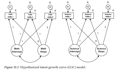
In reviewing this model, focus first on the six observed variables enclosed in rectangles at the top of the path diagram. Each variable con­stitutes a subscale score at one of three time points, with the first three representing perceived math ability and the latter three perceived science ability. Associated with each of these observed measures is their match­ing random measurement error term (E1-E6). (Disregard, for now, the numerals associated with these parameters; they are explained later in the chapter.) Moving down to the bottom of the diagram, we find two latent factors associated with each of these math and science domains; these fac­tors represent the Intercept and Slope for perceived math and science abil­ity, respectively.

Let’s turn now to the modeled paths in the diagram. As usual, the arrows leading from each of the four factors to their related observed variables represent the regression of observed scores at each of three time points onto their appropriate Intercept and Slope factors. As usual, the arrows leading from the Es to the observed variables represent the influence of random measurement error. Finally, the modeled covariance between each pair of Intercept and Slope factors (for math and science ability) is assumed in the specification of a LGC model.

The numerical values assigned to the paths flow from the Intercept and Slope factors to the observed variables; these paths of course represent fixed parameters in the model. The 1s specified for the paths flowing from the Intercept factor to each of the observed variables indicate that each is constrained to a value of 1.0. This constraint reflects the fact that the inter­cept value remains constant across time for each individual (Duncan et al., 1999). The values of 0, 1, and 2 assigned to the Slope parameters represent Years 1, 2, and 3, respectively. These constraints address the issue of model identification; they also ensure that the second factor can be interpreted as a slope. Three important points are of interest with respect to these fixed slope values: First, technically speaking, the first path (assigned a zero value) is really nonexistent and, therefore, has no effect. Although it would be less confusing to simply eliminate this parameter, it has become customary to include this path in the model, albeit with an assigned value of zero (Bentler, 2005). Second, these values represent equal time inter­vals (one year) between measurements; had data collection taken place at unequal intervals, the values would need to be calculated accordingly (e.g., 6 months = .5). (For an example of needed adjustment to time points, see Byrne, Lam, & Fielding, 2008.) Third, the choice of fixed values assigned to the Intercept and Slope factor loadings is somewhat arbitrary, as any linear transformation of the time scale is usually permissible, and the spe­cific coding of time chosen determines the interpretation of both factors. The Intercept factor is tied to a time scale (Duncan et al., 1999) because any shift in fixed loading values on the Slope factor will necessarily modify the scale of time bearing on the Intercept factor which, in turn, will influence interpretations (Duncan et al., 1999). Relatedly, the variances and correla­tions among the factors in the model will change depending on the chosen coding (see, e.g., Bloxis & Cho, 2008).

In this section, our focus is on the modeling of intraindividual change. Within the framework of structural equation modeling, this focus is cap­tured by the measurement model, the portion of a model that incorporates only linkages between the observed variables and their underlying unob­served factors. As you are well aware by now, of primary interest in any measurement model is the strength of the factor loadings or regression paths linking the observed and unobserved variables. As such, the only parts of the model in Figure 11.1 that are relevant in the modeling of intraindividual change are the regression paths linking the six observed variables to four factors (two intercepts, two slopes), the factor variances and covariances, and the related measurement errors associated with these observed variables.

Essentially, we can think of this part of the model as an ordinary fac­tor analysis model with two special features. First, all the loadings are fixed—there are no unknown factor loadings. Second, the particular pat­tern of fixed loadings plus the mean structure allows us to interpret the factors as intercept and slope factors. As in all factor models, the present case argues that each adolescent’s perceived math and science ability scores, at each of three time points (Time 1=0; Time 2 = 1; Time 3 = 2), are a function of three distinct components: (a) a factor loading matrix of con­stants (1; 1; 1) and known time values (0; 1; 2) that remain invariant across all individuals, multiplied by (b) a latent growth curve vector containing individual-specific and unknown factors, here called individual growth parameters (Intercept, Slope), plus (c) a vector of individual-specific and unknown errors of measurement. Whereas the latent growth curve vector represents the within-person true change in perceived math and science ability over time, the error vector represents the within-person noise that serves to erode these true change values (Willett & Sayer, 1994).

In preparing for transition from the modeling of intraindividual change to the modeling of interindividual change, it is important that we review briefly the basic concepts underlying the analyses of mean and covariance structures in structural equation modeling. When population means are of no interest in a model, analysis is based on only covariance structure parameters. As such, all scores are considered to be deviations from their means and, thus, the constant term (represented as a in a regres­sion equation) equals zero. Given that mean values played no part in the specification of the Level 1 (or within-person) portion of our LGC model, only the analysis of covariance structures is involved. However, in moving to Level 2, the between-person portion of the model, interest focuses on mean values associated with the Intercept and Slope factors; these values in turn influence the means of the observed variables. Because both lev­els are involved in the modeling of interindividual differences in change, analyses are now based on both mean and covariance structures.

Modeling Interindividual Differences in Change

Level 2 argues that, over and above hypothesized linear change in per­ceived math and science ability over time, trajectories will necessarily vary across adolescents as a consequence of different intercepts and slopes. Within the framework of structural equation modeling, this portion of the model reflects the “structural model” component which, in general, por­trays relations among unobserved factors and postulated relations among their associated residuals. Within the more specific LGC model, however, this structure is limited to the means of the Intercept and Slope factors, along with their related variances, which in essence represent deviations from the mean. The means carry information about average intercept and slope values, while the variances provide information on individual dif­ferences in intercept and slope values. The specification of these param­eters, then, makes possible the estimation of interindividual differences in change.

Let’s now reexamine Figure 11.1, albeit in more specific terms in order to clarify information bearing on possible differences in change across time. Within the context of the first construct, perceived ability in math, interest focuses on five parameters that are key to determining between-person differences in change: two factor means (Intercept; Slope), two factor vari­ances, and one factor covariance. The factor means represent the average population values for the Intercept and Slope and answer the question, “What is the population mean starting point and mean increment in Perceived Math Ability from Grades 8 through 10?” The factor variances represent deviations of the individual Intercepts and Slopes from their population means thereby reflecting population interindividual differ­ences in the initial (Grade 8) Perceived Math Ability scores, and the rate of change in these scores, respectively. Addressing the issue of variability, these key parameters answer the question, “Are there interindividual dif­ferences in the starting point and growth trajectories of Perceived Math Ability in the population?” Finally, the factor covariance represents the population covariance between any deviations in initial status and rate of change and answers the question, “Do students who start higher (or lower) in Perceived Math Ability tend to grow at higher (or lower) rates in that ability?”

Now that you have a basic understanding of LGC modeling, in gen­eral, and as it bears specifically on our hypothesized dual-domain model presented in Figure 11.1, let’s direct our attention now on both the mod­eling and testing of this model within the framework of Amos Graphics.

4. Testing Latent Growth Curve Models:

A Dual-Domain Model

The Hypothesized Model

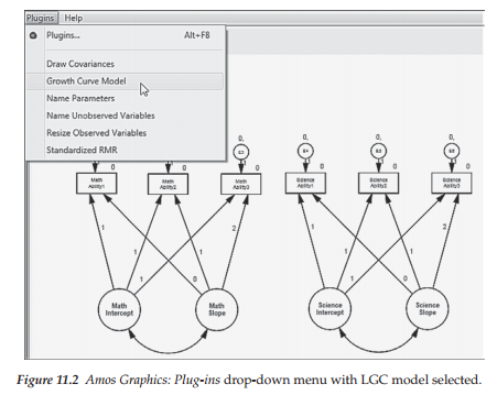
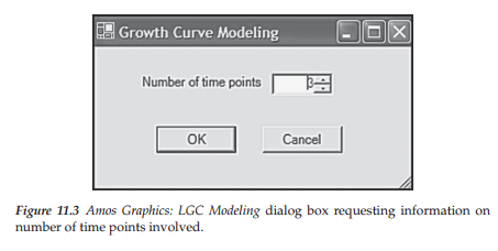
In building a LGC model using Amos Graphics, the program provides what it terms a Plug-in, an option that serves as a starter kit in providing the basic model and associated parameter specification. To use this Plug-in, click on the Plug-in menu and select Growth Curve Model, as shown in Figure 11.2. Once you make this selection and click on this growth curve option, the program asks if you wish to save the existing model. Once you say yes, the model disappears and you are presented with a blank page accompanied by a dialog box concerning the number of time points to be used in the analysis. Shown in Figure 11.3, however, is the number 3, which is the default value as it represents the minimal appropriate num­ber for LGC modeling.

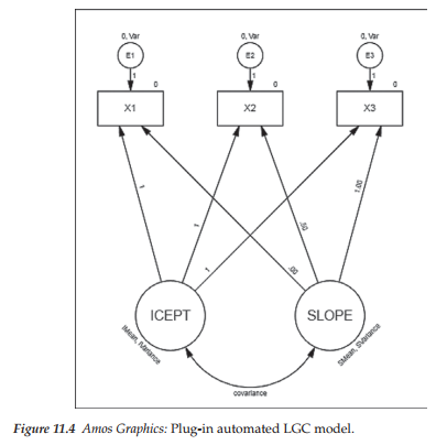
Shown in Figure 11.4 is the automated LGC model that appears fol­lowing the two previous steps. Simply duplicating this model allows for its application to the dual-domain model tested in this chapter. Importantly, however, there are several notations on this model that I consider to be inappropriate specifications for our hypothesized model. As a result, you will note their absence from the model portrayed in Figure 11.1. (These modifications are easily implemented via the Object Properties dialog box as has been demonstrated elsewhere in this volume and are shown below in Figures 11.5 and 11.8.) First, associated with each of the three error terms you will see a zero value, followed by a comma and the let­ters “Var.” As you know from Chapter 8, the first of these represents the mean and the second represents the variance of each error term. As per Amos Graphics notation, these labels indicate that the means of all error terms are constrained to zero and their variances are constrained equal across time. However, because specification of equivalent error variances would be inappropriate in the testing of our hypothesized model these labels are not specified in Figure 11.1. Indeed, error variances contribute importantly to the interpretation of model parameters through correction for measurement error associated with the variances of the Intercept and Slope factors. In other words, specification of error variance allows for the same basic interpretation of model parameters, albeit with correction for random measurement error (Duncan et al., 2006). Indeed, the error vari­ance equalities specified in the automated model are likely intended to offset an otherwise condition of model underidentification.

A second change between the model shown in Figure 11.1 and that of Figure 11.4 involves labels associated with the latent factors. On the automated model, you will note the labels, IMean, Variance, SMean, and SVariance associated with the Intercept and Slope factors, respectively.

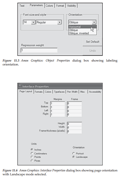
Again, these labels signal that these factor parameters are constrained equal across time. Because these constraint specifications are inappro­priate for our analyses, they are not included in our specified model (Figure 11.1). Third, note that the paths leading from the Slope factor to the observed variable for each time point are numbered .00, .50, and 1.00, whereas these path parameters in our hypothesized model are numbered 0, 1, 2 in accordance with the time lag between data collections. Finally, of a relatively minor note, is a change in orientation of the numbers assigned to the Intercept and Slope paths from oblique to horizontal (see Figure 11.5).

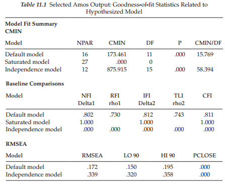
Before moving on to the analyses for this chapter, it may be instruc­tive for me to alert you to a couple of additional considerations related to the specification of LGC models. As is typical for these models, you will likely want to orient your page setup to landscape mode. Implementation of this reorientation is accomplished via the Interface Properties dialog box as illustrated in Figure 11.6; its selection is made from the View drop-down menu.

Following this long but nonetheless essential overview of the mod­eling and testing of LGC models using Amos Graphics, we are now ready to test the model shown in Figure 11.1 and examine the results.

Selected Amos Output: Hypothesized Model

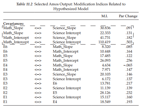
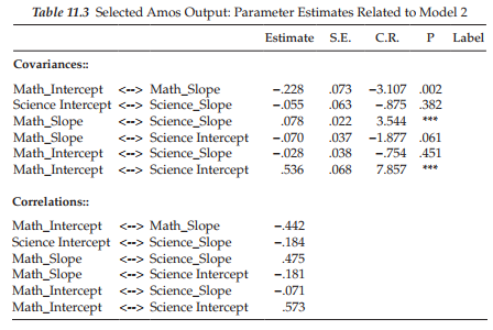
Of prime importance in testing this first model are the extent to which it fits the data and the extent to which it may need some modification. We turn first to the goodness-of-fit statistics reported in Table 11.1. Of key concern here is the obviously poor fit of the model as indicated by the CFI value of .811 and the RMSEA value of .172. Clearly this model is misspeci- fied in a very major way. For answers to this substantial misspecification, let’s review the modification indices, which are reported in Table 11.2. Of primary interest are misspecification statistics associated with the two intercept and two slope factors, which have been highlighted within the broken-line rectangle.

In reviewing these modification indices, we see that not including a covariance between the Math Ability and Science Ability Intercept factors is accounting for the bulk of the misspecification. Given the fairly substantial modification indices associated with the remaining three fac­tor covariances, together with Willet and Sayer’s (1996) caveat that, in multiple-domain LGC models, covariation among the growth parameters across domains should be considered, I respecified a second model (Model 2) in which all four factor covariances were specified. These results, as they relate to the parameter estimates, are reported in Table 11.3.

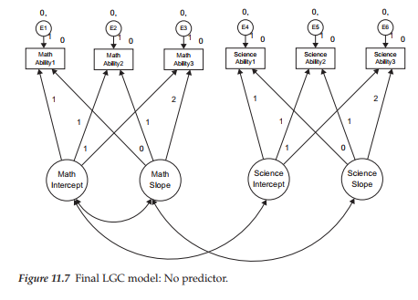
Although goodness-of-fit results pertinent to Model 2 were substan­tially improved (x²(₇) = 32.338; CFI = .971; RMSEA = .085), a review of the estimates related to these factor covariances revealed only three to be sta­tistically significant and thus worthy of incorporation into the final model. Specifically, results revealed the covariance between the Math Ability and Science Ability Intercept factors and between their related Slope factors to be important parameters in the model. In addition, given a probability value <.05 for the covariance between the Math Ability Intercept and the Science Ability Slope, I considered it important also to include this param­eter in the final model. The remaining three statistically nonsignificant fac­tor covariances were deleted from the model. This final model (Model 3) is shown schematically in Figure 11.7.

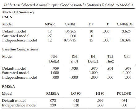
Of substantial interest in our review of results pertinent to this model is what a difference the incorporation of two additional factor covariances can make! As shown in Table 11.4, we now find a nice well-fitting model with related fit statistics of: x²(₁₀) = 32.338, CFI = .969, and RMSEA = .073. Having now determined a well-fitting model, we are ready to review the substantive results of the analysis. Both the unstandardized and standard­ized parameter estimates are reported in Table 11.5.

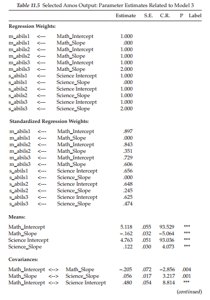
Given that the regression weights represented only fixed parame­ters, there is little interest in this section. Of major importance, however, are the estimates reported in the remaining sections of the output file. Turning first to the Means estimates, we see that these parameters for both the Intercepts and Slopes were statistically significant. Specifically, findings reveal the average score for Perceived Science Ability (4.763) to be slightly lower than for Perceived Math Ability (5.118). However, whereas adolescents’ average self-perceived Math Ability scores decreased over a 3-year period from Grade 8 to Grade 10 (as indicated by the a value of -0.162), those related to self-perceived Science Ability increased (0.122).

Let’s turn now to the factor covariances, reviewing first, the within-domain covariance, that is to say, the covariance between the inter­cept and slope related to the same construct. Here, we find the estimated covariance between the Intercept and Slope factors for Math Ability to be statistically significant (p < .05). The negative estimate of -.205 suggests that adolescents whose self-perceived scores in math ability were high in Grade 8 demonstrated a lower rate of increase in these scores over the 3-year period from Grade 8 through Grade 10 than was the case for ado­lescents whose self-perceived math ability scores were lower at Time 1. In other words, Grade 8 students who perceived themselves as being less able in math than their peers, made the greater gains. A negative corre­lation between initial status and possible gain is an old phenomenon in psychology known as the law of initial values.

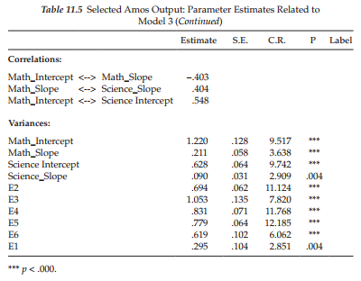
Turning to the first between-domain covariance shown in the output (Math Slope/Science Slope), we see that, although statistically significant, this reported value is small (.056). Nonetheless, a review of the stand­ardized coefficients show this correlation (r = .404), as for the other two covariances, to be moderately high. This result indicates that as growth in adolescents’ perceptions of their math ability from grades 8 through 10 undergoes a moderate increase, so also do their perceptions of science ability. Finally, the fairly strong correlation between Intercepts related to Math Ability and Science Ability (r = .548) indicates that adolescents per­ceiving themselves as having high ability in math also view themselves concomitantly as having high ability in science.

Finally, turning to the Variance section of the output file, we note that, importantly, all estimates related to the Intercept and Slope for each per­ceived ability domain are statistically significant (p < .05). These findings reveal strong interindividual differences in both the initial scores of per­ceived ability in math and science at Time 1, and in their change over time, as the adolescents progressed from Grade 8 through Grade 10. Such evi­dence of interindividual differences provides powerful support for further investigation of variability related to the growth trajectories. In particular, the incorporation of predictors into the model can serve to explain their variability. Of somewhat less importance substantively, albeit important methodologically, all random measurement error terms are also statisti­cally significant (p < .05).

4. Testing Latent Growth Curve Models: Gender as a Time-invariant Predictor of Change

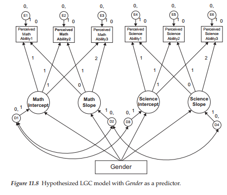
As noted earlier, provided with evidence of interindividual differences, we can then ask whether, and to what extent, one or more predictors might explain this heterogeneity. For our purposes here, we ask whether statistically significant heterogeneity in the individual growth trajectories (i.e., intercept and slope) of perceived ability in math and science can be explained by gender as a time-invariant predictor of change. As such, two questions that we might ask are: “Do self-perceptions of ability in math and science differ for adolescent boys and girls at Time 1 (Grade 8)?” and “Does the rate at which self-perceived ability in math and science change over time differ for adolescent boys and girls?” To answer these questions, the predictor variable “gender” must be incorporated into the Level 2 (or structural) part of the model. This predictor model represents an extension of our final best-fitting multiple domain model (Model 3) and is shown schematically in Figure 11.8.

Of import regarding the path diagram displayed in Figure 11.8 is the addition of four new model components. First, you will note the four regression paths that flow from the variable of “Gender” to the Intercept and Slope factors associated with the Math Ability and Science Ability domains. These regression paths are of primary interest in this predictor model as they hold the key in answering the question of whether the tra­jectory of perceived ability in math and science differs for adolescent boys and girls. Second, there is now a latent residual associated with each of the Intercept and Slope factors. This addition is a necessary requirement as these factors are now dependent variables in the model due to the regres­sion paths generated from the predictor variable of gender. Because the
variance of dependent variables cannot be estimated in structural equa­tion modeling, the latent factor residuals serve as proxies for the Intercept and Slope factors in capturing these variances. These residuals now rep­resent variation remaining in the Intercepts and Slopes after all variabil­ity in their prediction by gender has been explained (Willett & Keiley, 2000). Rephrased within a comparative framework, we note that for the dual-domain model in which no predictors were specified, the residuals represented deviations between the factor Intercepts and Slopes, and their population means. In contrast, for this current model in which a predic­tor variable is specified, the residual variances represent deviations from their conditional population means. As such, these residuals represent the adjusted values of factor Intercepts and Slopes after partialling out the linear effect of the gender predictor variable (Willett & Keiley, 2000). Third, the double-headed arrows representing the factor covariances are now shown linking the appropriate residuals rather than the factors them­selves. Finally, the means of the residuals are fixed to 0.0, as indicated by the assigned 0 followed by a comma.

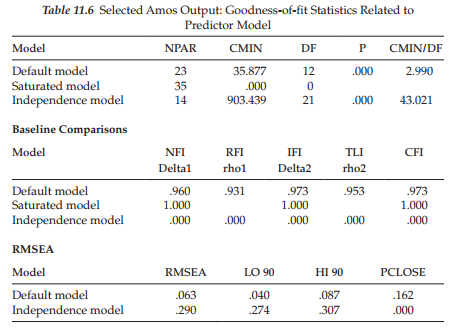
Let’s turn now to the goodness-of-fit findings resulting from the test of this predictor model as summarized in Table 11.6. Interestingly, here we find evidence of an extremely well-fitting model more than is even bet­ter than the final LGC model having no predictor variable (x²(₁₂) = 35.887; CFI = .973; RMSEA = .063).

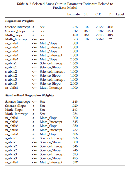
Parameter estimates related to this predictor model are presented in Table 11.7. However, because the content of major import related to this model focuses on the variable of Gender, the results presented are perti­nent only to the related regression paths and their weights.⁴ Turning first to results for Perceived Math Ability, we see that Gender was found to be a statistically significant predictor of both initial status (.563) and rate of change (-.150) at p < .05. Given a coding of “0” for females and “1” for males, these findings suggest that, whereas self-perceived ability in math was, on average, higher for boys than for girls by a value of .563 at Time 1, the rate of change in this perception for boys, from Grade 8 through Grade 10, was slower than it was for girls by a value of .150. (The negative coef­ficient indicates that boys had the lower slope.)

Results related to Perceived Science Ability again revealed Gender to be a significant predictor of Perceived Science Ability in Grade 8, with boys showing higher scores on average than girls by a value of .226 (p < .05). On the other hand, rate of change was found to be indistinguishable between boys and girls as indicated by its nonsignificant estimate (p = .774).

To conclude, I draw from the work of Willett and Sayer (1994, 1996) in highlighting several important features captured by the LGC model­ing approach to the investigation of change. First, the methodology can accommodate anywhere from 3 to 30 waves of longitudinal data equally well. Willett (1988, 1989) has shown, however, that the more waves of data collected, the more precise will be the estimated growth trajectory and the higher will be the reliability for the measurement of change. Second, there is no requirement that the time lag between each wave of assessments be equivalent. Indeed, LGC modeling can easily accommodate irregularly spaced measurements, but with the caveat that all subjects are measured on the same set of occasions. Third, individual change can be represented by either a linear or a nonlinear growth trajectory. Although linear growth is typically assumed by default, this assumption is easily tested and the model respecified to address curvilinearity if need be. Fourth, in contrast to traditional methods used in measuring change, LGC models allow not only for the estimation of measurement error variances, but also, for their autocorrelation and fluctuation across time in the event that tests for the assumptions of independence and homoscedasticity are found to be untenable. Fifth, multiple predictors of change can be included in the LGC model. They may be fixed, as in the specification of gender in the pre­sent chapter, or they may be time-varying (see, e.g., Byrne, 2008; Willett & Keiley, 2000). Finally, the three key statistical assumptions associated with our application of LGC modeling (linearity; independence of measure­ment error variances; homoscedasticity of measurement error variances), although not demonstrated in this chapter, can be easily tested via a com­parison of nested models (see Byrne & Crombie, 2003).

A classic example of LGC modeling typically represents a linear change process comprised of two latent growth factors: (a) an intercept that describes an initial time point, and (b) a linear slope that summarizes constant change over time (Kohli & Harring, 2013). This was the case of the example application presented in this chapter, albeit with the excep­tion of a dual-, rather than a single-domain framework. For readers wish­ing to become more familiar with these basic processes, in addition to how to deal with other important issues such as incomplete data, nonlinear growth models, and the inclusion of group comparisons and treatment effects, I highly recommend the nonmathematical coverage of these topics by McArdle (2012). Still other topics that may be of interest are the issue of data that comprise heterogeneous subgroups, rather than a single homog­enous population (the usual case) (see Hwang, Takane, & DeSarbo, 2007), and the determination of power in growth curve modeling (see Hertzog, von Oertzen, Ghisletta, & Lindenberger, 2008). Finally, in the interest of completeness I consider it important to make you aware that multilevel models provide an alternative way to study change with structural mod­els (see, e.g., Bovaird, 2007; Duncan et al., 2006; Singer & Willett, 2003).

Source: Byrne Barbara M. (2016), Structural Equation Modeling with Amos: Basic Concepts, Applications, and Programming, Routledge; 3rd edition.