Application 10: Use of Bootstrapping in Addressing Nonnormal Data with AMOS

1. Key Concepts

• SEM assumption of multivariate normality
• Concept of bootstrapping
• Benefits, limitations, and caveats related to bootstrapping
• Nonparametric (simple, naive) bootstrap
• Sample ML estimates versus bootstrap Ml estimates
• Bollen-Stine bootstrap option

Two critically important assumptions associated with structural equation modeling (SEM) in the analysis of covariance and mean structures are that the data be of a continuous scale and that they have a multivariate normal distribution. These underlying assumptions are linked to large-sample (i.e., asymptotic) theory within which SEM is embedded. More specifi­cally, they derive from the approach taken in the estimation of param­eters using the SEM methodology. In the early days of SEM (1970s to early 1980s), either maximum likelihood (ML) or normal theory generalized least squares (GLS) estimation were typically used, both of which demand that the data be continuous and multivariate normal. However, beginning in the 1980s, primarily in response to mass criticism of SEM research that failed to meet these assumptions, there was a movement on the part of statistical methodologists to develop estimators capable of being used with data that were (a) multivariate nonnormal and (b) of a categorical or ordinal nature (Matsueda, 2012). Beginning with the development of the asymptotic distribution-free (ADF) (Browne, 1984) and elliptical estima­tors, this work grew to include robust ML estimators capable of taking the nonnormality of the data and categorical nature of the data into account and adjusting the estimates accordingly (see Chapters 3 and 5 of this vol­ume). Although these robust estimators are available in other SEM pro­grams (e.g., EQS [Bentler, 2005]; Mplus [Muthen & Muthen, 1998-2012]),¹ unfortunately they are not incorporated into the Amos program. Thus, other methods of addressing these concerns must be used. In Chapter 5,

I outlined the Bayesian approach taken by Amos in dealing with categor­ical data. In this chapter, I describe and illustrate the use of bootstrap­ping in addressing the issue of multivariate nonnormal data. However, for a more extensive overview of bootstrapping used within this context, I highly recommend a very clearly written and nonmathematically pre­sented book chapter by Hancock and Liu (2012).

Despite the importance of normality for all parametric statistical ana­lyses, a review of the literature provides ample evidence of empirical research wherein the issue of distributional normality has been blatantly ignored. For example, in an analysis of 440 achievement and psychomet­ric data sets, all of which exceeded a sample size of 400, Micceri (1989) reported that the majority of these data failed to follow either a univari­ate or multivariate normal distribution. Furthermore, he found that most researchers seemed to be totally oblivious even to the fact that they had violated this statistical assumption (see also, Zhu, 1997). Within the more limited context of the SEM literature, it is easy to find evidence of the same phenomenon. As a case in point we can turn to Breckler (1990), who iden­tified 72 articles appearing in personality and social psychology journals between the years 1977 and 1987 that employed the SEM methodology. His review of these published studies revealed that only 19% actually acknowledged the normal theory assumptions, and fewer than 10% expli­citly tested for their possible violation.

Following a review of empirical studies of nonnormality in SEM, West et al. (1995) summarized four important findings. First, as data become increasingly nonnormal, the x² value derived from both ML and GLS esti­mation becomes excessively large. The consequence of this situation is that it encourages researchers to seek further modification of their hypoth­esized model in an effort to attain adequate fit to the data. However, given the spuriously high x² value, these efforts can lead to inappropriate and nonreplicable modifications to otherwise theoretically adequate models (see also, MacCallum, Roznowski, & Necowitz, 1992; Lei & Lomax, 2005). Second, when sample sizes are small (even in the event of multivariate normality), both the ML and GLS estimators yield x² values that are some­what inflated. Furthermore, as sample size decreases and nonnormality increases, researchers are faced with a growing proportion of analyses that fail to converge or that result in an improper solution (see Anderson & Gerbing, 1984; Boomsma, 1982). Third, when data are nonnormal, fit indices such as the Tucker-Lewis Index (TLI: Tucker & Lewis, 1973) and the Comparative Fit Index (CFI; Bentler, 1990) yield values that are mod­estly underestimated (see also Marsh, Balla, & McDonald, 1988). Finally, nonnormality can lead to spuriously low standard errors, with degrees of underestimation ranging from moderate to severe (Chou et al., 1991; Finch et al., 1997). The consequences here are that because the standard errors are underestimated, the regression paths and factor/error covari­ances will be statistically significant, although they may not be so in the population.

Given that, in practice, most data fail to meet the assumption of multi­variate normality, West et al. (1995) noted increasing interest among SEM researchers in (a) establishing the robustness of SEM to violations of the normality assumption, and (b) developing alternative reparatory strat­egies when this assumption is violated. Particularly troublesome in SEM analyses is the presence of excessive kurtosis (see, e.g., Bollen & Stine, 1993; West et al., 1995). In a very clearly presented review of both the problems encountered in working with multivariate nonnormal data in SEM and the diverse remedial options proposed for their resolution, West and colleagues provide the reader with a solid framework within which to comprehend the difficulties that arise. I highly recommend their book chapter to all SEM researchers, with double emphasis for those who may be new to this methodology.

One approach to handling the presence of multivariate nonnormal data is to use a procedure known as “the bootstrap” (Hancock & Liu, 2012; West et al., 1995; Yung & Bentler, 1996; Zhu, 1997). This technique was first brought to light by Efron (1979, 1982) and has been subsequently high­lighted by Kotz and Johnson (1992) as having had a significant impact on the field of statistics. The term “bootstrap” derives from the expression “to pull oneself up by the bootstraps,” reflecting the notion that the origi­nal sample gives rise to multiple additional ones. As such, bootstrapping serves as a resampling procedure by which the original sample is consid­ered to represent the population. Multiple subsamples of the same size as the parent sample are then drawn randomly, with replacement, from this population and provide the data for empirical investigation of the vari­ability of parameter estimates and indices of fit. For very comprehensible introductions to the underlying rationale and operation of bootstrapping, readers are referred to Hancock and Liu (2012), Diaconis and Efron (1983), Stine (1990), and Zhu (1997).

Prior to the advent of high-speed computers, the technique of boot­strapping could not have existed (Efron, 1979). In fact, it is for this very reason that bootstrapping has been categorized as a computer-intensive statistical procedure in the literature (see, e.g., Diaconis & Efron, 1983; Noreen, 1989). Computer-intensive techniques share the appealing fea­ture of being free from two constraining statistical assumptions generally associated with the analysis of data: (a) that the data are normally dis­tributed, and (b) that the researcher is able to explore more complicated problems, using a wider array of statistical tools than was previously pos­sible (Diaconis & Efron, 1983). Before turning to our example application in this chapter, let’s review, first, the basic principles associated with the bootstrap technique, its major benefits and limitations, and finally, some caveats bearing on its use in SEM.

2. Basic Principles Underlying the Bootstrap Procedure

The key idea underlying the bootstrap technique is that it enables the researcher to create multiple subsamples from an original data base. The importance of this action is that one can then examine parameter distributions relative to each of these spawned samples. Considered cumulatively, these distributions serve as a bootstrap sampling dis­tribution that technically operates in the same way as does the sam­pling distribution generally associated with parametric inferential statistics. In contrast to traditional statistical methods, however, the bootstrapping sampling distribution is concrete and allows for com­parison of parametric values over repeated samples that have been drawn (with replacement) from the original sample. With traditional inferential procedures, on the other hand, comparison is based on an infinite number of samples drawn hypothetically from the popu­lation of interest. Of import here is the fact that the sampling dis­tribution of the inferential approach is based on available analytic formulas that are linked to assumptions of normality, whereas the bootstrap sampling distribution is rendered free from such restric­tions (Zhu, 1997).

To give you a general flavor of how the bootstrapping strategy oper­ates in practice, let’s examine a very simple example. Suppose that we have an original sample of 350 cases; the computed mean on variable X is found to be 8.0, with a standard error of 2.5. Then, suppose that we have the computer generate 200 samples consisting of 350 cases each by randomly selecting cases with replacement from the original sample. For each of these subsamples, the computer will record a mean value, com­pute the average mean value across the 200 samples, and calculate the standard error.

Within the framework of SEM, the same procedure holds, albeit one can evaluate the stability of model parameters, and a wide variety of other estimated quantities (Kline, 2011; Stine, 1990; Yung & Bentler, 1996). Furthermore, depending on the bootstrapping capabilities of the particular computer program in use, one may also test for the stability of goodness-of-fit indices relative to the model as a whole (Bollen & Stine, 1993; Kline, 2011). Amos can provide this information. (For an evaluative review of the application and results of bootstrapping to SEM models, readers are referred to Yung and Bentler [1996].)

Benefits and Limitations of the Bootstrap Procedure

The primary advantage of bootstrapping, in general, is that it allows the researcher to assess the stability of parameter estimates and thereby report their values with a greater degree of accuracy. As Zhu (1997, p. 50) noted, in implied reference to the traditional parametric approach, “it may be better to draw conclusions about the parameters of a population strictly from the sample at hand … , than to make perhaps unrealistic assumptions about the population.” Within the more specific context of SEM, the boot­strap procedure provides a mechanism for addressing situations where the ponderous statistical assumptions of large sample size and multivari­ate normality may not hold (Yung & Bentler, 1996). Perhaps the strongest advantage of bootstrapping in SEM is “its ‘automatic’ refinement on stand­ard asymptotic theories (e.g., higher-order accuracy) so that the bootstrap can be applied even for samples with moderate (but not extremely small) sizes” (Yung & Bentler, 1996, p. 223).

These benefits notwithstanding, the bootstrap procedure is not with­out its limitations and difficulties. Of primary interest, are four such limi­tations. First, the bootstrap sampling distribution is generated from one “original” sample that is assumed to be representative of the population. In the event that such representation is not forthcoming, the bootstrap procedure will lead to misleading results (Zhu, 1997). Second, Yung and Bentler (1996) have noted that, in order for the bootstrap to work within the framework of covariance structure analysis, the assumption of inde­pendence and identical distribution of observations must be met. They contend that such an assumption is intrinsic to any justification of replace­ment sampling from the reproduced correlation matrix of the bootstrap. Third, the success of a bootstrap analysis depends on the degree to which the sampling behavior of the statistic of interest is consistent when the samples are drawn from the empirical distribution and when they are drawn from the original population (Bollen & Stine, 1993). Finally, when data are multivariate normal, the bootstrap standard error estimates have been found to be more biased than those derived from the standard ML method (Ichikawa & Konishi, 1995). In contrast, when the underlying dis­tribution is nonnormal, the bootstrap estimates are less biased than they are for the standard ML estimates.

Caveats Regarding the Use of Bootstrapping in SEM

Although the bootstrap procedure is recommended for SEM as an approach to dealing with data that are multivariate nonnormal, it is important that researchers be cognizant of its limitations in this regard as well as of its use in addressing issues of small sample size and lack of independent samples for replication (Kline, 2011). Findings from Monte Carlo simulation stud­ies of the bootstrap procedures have led researchers to issue several cave­ats regarding its use. Foremost among such caveats is Yung and Bentler’s (1996) admonition that bootstrapping is definitely not a panacea for small samples. Because the bootstrap sample distributions depend heavily on the accuracy of estimates based on the parent distribution, it seems evident that such precision can only derive from a sample that is at least moder­ately large (see Ichikawa & Konishi, 1995; Yung & Bentler, 1994).

A second caveat addresses the adequacy of standard errors derived from bootstrapping. Yung and Bentler (1996) exhort that, although the bootstrap procedure is helpful in estimating standard errors in the face of nonnormal data, it should not be regarded as the absolutely only and best method. They note that researchers may wish to achieve particular statis­tical properties such as efficiency, robustness, and the like and, thus, may prefer using an alternate estimation procedure.

As a third caveat, Yung and Bentler (1996) caution researchers against using the bootstrap procedure with the naive belief that the results will be accurate and trustworthy. They point to the studies of Bollen and Stine (1988, 1993) in noting that, indeed, there are situations where bootstrap­ping simply will not work. The primary difficulty here, however, is that there is as yet no way of pinpointing when and how the bootstrap proced­ure will fail. In the interim, we must await further developments in this area of SEM research.

Finally, Arbuckle (2007) admonishes that when bootstrapping is used to generate empirical standard errors for parameters of interest in SEM, it is critical that the researcher constrain to some nonzero value, one factor loading path per factor, rather than the factor variance in the process of establishing model identification. Hancock and Nevitt (1999) have shown that constraining factor variances to a fixed value of 1.0, in lieu of one fac­tor loading per congeneric set of indicators, leads to bootstrap standard errors that are highly inflated.

At this point, hopefully you have at least a good general idea of the use of bootstrapping within the framework of SEM analyses. However, for more in-depth and extensive coverage of bootstrapping, readers are referred to Chernick (1999) and Lunnenborg (2000). With this background information in place, then, let’s move on to an actual application of the bootstrap procedure.

3. Modeling with Amos Graphics

When conducting the bootstrap procedure using Amos Graphics, the researcher is provided with one set of parameter estimates, albeit two sets of their related standard errors. The first set of estimates is part of the regular Amos output when ML or GLS estimation is requested. The calcu­lation of these standard errors is based on formulas that assume a multi­variate normal distribution of the data. The second set of estimates derives from the bootstrap samples and, thus, is empirically determined. There are several types of bootstrapping, but the general approach to this pro­cess described here is commonly termed as simple, nonparametric, or naive bootstrapping (Hancock & Liu, 2012). The advantage of bootstrapping, as discussed above, is that it can be used to generate an approximate stand­ard error for many statistics that Amos computes, albeit without having to satisfy the assumption of multivariate normality. It is with this beneficial feature in mind, that we review the present application.

The Hypothesized Model

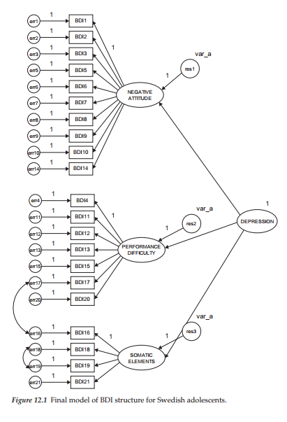
The model to be used in demonstrating the bootstrap procedure represents a second-order CFA model akin to the one presented in Chapter 5 in that it also represents the Beck Depression Inventory (BDI). However, whereas analyses conducted in Chapter 5 were based on the revised version of the BDI (Beck et al., 1996), those conducted in this chapter are based on the original version of the instrument (Beck et al., 1961). The sample data used in the current chapter represent item scores for 1,096 Swedish adolescents. The purpose of the original study from which this application is taken was to demonstrate the extent to which item score data can vary across culture despite baseline models that (except for two correlated errors) were struc­turally equivalent (see Byrne & Campbell, 1999). Although data pertinent to Canadian (n = 658) and Bulgarian (n = 691) adolescents were included in the original study, we focus our attention on only the Swedish group in the present chapter. In particular, we examine bootstrap samples related to the final baseline model for Swedish adolescents, which is displayed in Figure 12.1.

Characteristics of the Sample

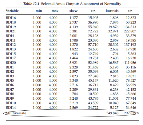
Of import in this bootstrapping example is that despite the adequately large size of the Swedish sample, the data are severely nonnormally dis­tributed. Univariate skewness (SK) values ranged from 0.784 to 5.381, with a mean SK of 2.603; univariate kurtosis (KU) values ranged from 0.794 to 32.971, with a mean KU of 8.537. From a multivariate perspec­tive, Mardia’s (1970, 1974) normalized estimate of multivariate kurtosis was found to be 292.839. Based on a very large sample that is multivariate normal, this estimate is distributed as a unit normal variate (Bentler, 2005). Thus, when estimated values are large, they indicate significant positive kurtosis. Indeed, Bentler (2005) has suggested that in practice, values >5.00 are indicative of data that are nonnormally distributed. Recall from the discussion of nonnormality in Chapter 4, that in Amos, the critical ratio can be considered to represent Mardia’s normalized estimate, although it is not explicitly labeled as such (J. Arbuckle, personal communication, March, 2014). Given a normalized Mardia estimated value of 292.839, then, there is no question that the data clearly are not multivariate normal.

Applying the Bootstrap Procedure

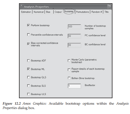
Application of the bootstrap procedure, using Amos, is very easy and straightforward. With the model shown in Figure 12.1 open, all that is needed is to access the Analysis Properties dialog box, either from the pull-down menu or by clicking on its related icon (5M). Once this dialog box has been opened, you simply select the Bootstrap tab shown encircled in Figure 12.2. Noting the checked boxes, you will see that I have requested Amos to perform a bootstrap on 500 samples using the ML estimator, and to provide bias-corrected confidence intervals for each of the parameter bootstrap estimates; the 90% level is default. As you can readily see in Figure 12.2, the program provides the researcher with several choices regarding estimators in addition to options related to (a) Monte Carlo bootstrapping, (b) details related to each bootstrap sample, (c) use of the Bollen-Stine bootstrap, and (d) adjusting the speed of the bootstrap algo­rithm via the Bootfactor.

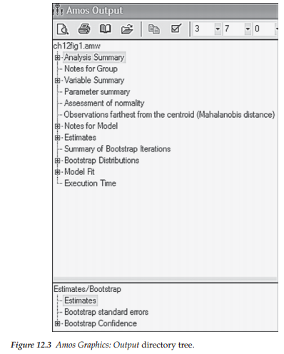
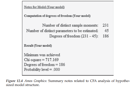
Once you have made your selections on the Bootstrap tab, you are ready to execute the job. Selecting “Calculate Estimates” either from the Model-Fit pull-down menu, or by clicking on the icon (E) sets the bootstrapping action in motion. Figure 12.3 shows the Amos Output file directory tree that appears once the execution has been completed. In reviewing this set of output sections, it is worth noting the separation of the usual model information (upper section) and the bootstrap informa­tion (lower section). As can be seen in the summary notes presented in Figure 12.4, there were no estimation problems (minimum was achieved), the x² value is reported as 717.2, with 186 degrees of freedom.

4. Selected Amos Output

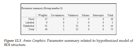
We now review various components of the Amos text output, turning first to the Parameter summary, which is presented in Figure 12.5.

Parameter Summary

Although, by now, you will likely have no difficulty interpreting the Parameter summary, I would like to draw your attention to the three labeled parameters listed in the “Variances” column. These variances per­tain to the three residual errors that, as in Chapter 5, were constrained to be equal. For safe measure, let’s review the last column, which reports the total number of fixed, labeled, and unlabeled parameters in the model. Details related to the remainder of this summary are as follows:

• 28 fixed parameters: 21 regression paths (or weights) associated with the measurement error terms, 3 associated with the residual terms,and 3 associated with the first factor loading of each congeneric set of indicator measures; 1 variance fixed to 1.0 associated with the higher-order factor.

• 44 unlabeled (estimated) parameters: 21 factor loadings (18 first-order; 3 second-order); 2 covariances (2 correlated errors); 21 variances (measurement error terms).

Assessment of Normality

Given the extreme nonnormality of these data, I consider it important that you have the opportunity to review this information as reported in the output file. This information is accessed by checking the “Normality/ Outliers” option found on the Estimation tab of the Analysis Properties dialog box (see Chapter 4). As indicated by the labeling of this option, Amos presents information related to the normality of the data from two perspectives—one indicative of the skewness and kurtosis of each param­eter, the other of the presence of outliers. We turn first to the skewness and kurtosis issue.

Statistical evidence of nonnormality. Although this information was sum­marized above, the output presented in Table 12.1 enables you to review skewness and kurtosis values related to each BDI item. As noted earlier, the multivariate value of 549.848 represents Mardia’s (1970) coefficient of multivariate kurtosis, the critical ratio of which is 292.839 and represents its normalized estimate.

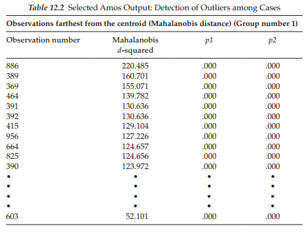
Statistical evidence of outliers. In addition to statistical information related to skewness and kurtosis, Amos provides information related to possible outliers in the data. This option is labeled on the Output directory tree as “Observations farthest from the centroid (Mahalanobis distance)” (see Figure 12.3). As such, the program identifies any case for which the observed scores differ markedly from the centroid of scores for all 1,096 cases; Mahalanobis d-squared values are used as the measure of distance and they are reported in decreasing rank order. This information is presented in Table 12.2 for the first 11 and final ranked scores. Here we see that Case #886 is the farthest from the centroid with a Mahalanobis d² value of 220.485; this value is then followed by two columns, pi and p2. The pi column indi­cates that, assuming normality, the probability of d² (for Case #886) exceeding a value of 220.485 is <.000. The p2 column, also assuming normality, reveals that the probability is still <.000 that the largest d² value for any individual case would exceed 220.485. Arbuckle (2015) notes that, while small num­bers appearing in the first column (pi) are to be expected, small numbers in the second column (p2) indicate observations that are improbably far from the centroid under the hypothesis of normality. Given the wide gap in Mahalanobis d² values between Case #886 and the second case (#389), rela­tive to all other cases, I would judge Case #886 to be an outlier and would consider deleting this case from further analyses. Indeed, based on the same rationale of comparison, I would probably delete the next three cases as well.

Parameter Estimates and Standard Errors

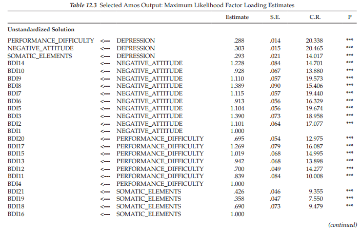
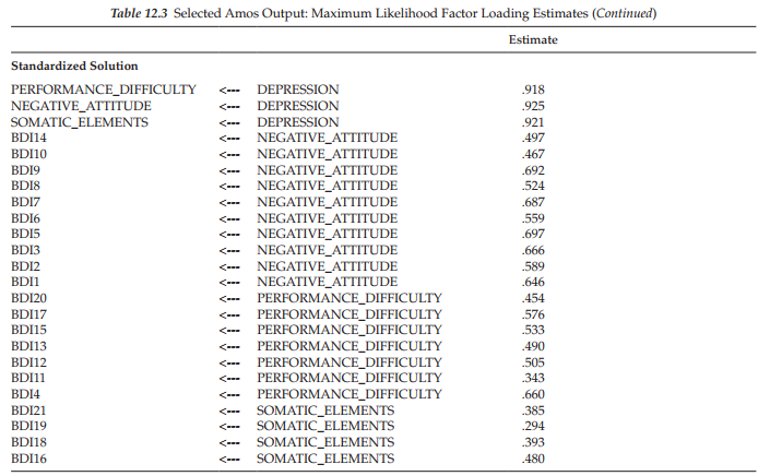
When bootstrapping is requested, Amos provides two sets of informa­tion, as could be seen in the Output directory tree (see Figure 12.3); these include the regular ML parameter estimates, along with their standard errors (shown in the upper section of the tree), together with related boot­strap information (shown in the lower section of the tree). We turn first to the regular ML estimates, which are presented in Table 12.3.

Sample ML estimates and standard errors. In the interest of space, the unstandardized and standardized estimates for only the factor loadings (i.e., first- and second-order regression weights) are presented here. Of primary interest are the standard errors (SEs) as they provide the basis for determining statistical significance related to the parameter estimates (i.e., estimate divided by standard error equals the critical ratio). Importantly, then, these initial standard errors subsequently can be compared with those reported for the bootstrapped samples.

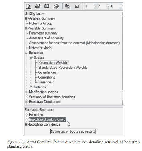
Bootstrap ML standard errors. Once the ML parameter estimates have been reported for the original sample of cases, the program then turns to results related to the bootstrap samples. Amos provides a summary of the bootstrap iterations, which can be accessed from the output directory tree. This option is visible in Figure 12.6, where it appears on the the last line in the upper section of the tree. The summary reports two aspects of the iteration process: (a) minimization history of the number of itera­tions required to fit the hypothesized model to the bootstrap samples, and (b) the extent to which the process was successful. This information perti­nent to the Swedish data is shown in Figure 12.7.

In reviewing Figure 12.7, you will note four columns. The first, labeled Iterations, reports that 19 iterations were needed to complete 500 bootstrap samples. The three method columns are ordered from left to right in terms of their speed and reliability. As such, minimization Method 0 is the slow­est and is not currently used in Amos 23; thus this column always contains 0s. Method 1 is reported in Amos documentation to be generally fast and reliable. Method 2 represents the most reliable minimization algorithm and is used as a follow-up method if Method 1 fails during the bootstrapping process.

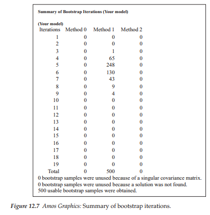
As evidenced from the information reported in Figure 12.7, Method 1 was completely successful in its task of bootstrapping 500 usable sam­ples; none was found to be unusable. The numbers entered in the Method 1 column represent the coordinate between number of bootstrap samples and number of iterations. For example, the number “65” on the fourth line indicates that for 65 bootstrap samples, Method 1 reached a minimum in 4 iterations. In contrast, Arbuckle (2015) notes that it is entirely possible that one or more bootstrap samples will have a singular matrix, or that Amos fails to find a solution for some samples. Should this occur, the program reports this occurrence and omits them from the bootstrap analysis.

In general, Hancock and Liu (2012) have noted that although the bootstrap standard errors tend not to perform as well as the ML standard errors given data that are multivariate normal, overall they comprise less bias than the original ML standard errors under a wide variety of non­normal conditions. Of critical importance, however, is the expectation that in the case of an original sample that either is small or is not continuously distributed (or both), one or more of the bootstrap samples is likely to yield a singular covariance matrix. In such instances, Amos may be unable to find a solution for some of the bootstrap samples. Given such findings, the program reports these failed bootstrap samples and excludes them from the bootstrap analysis (Arbuckle, 2015).

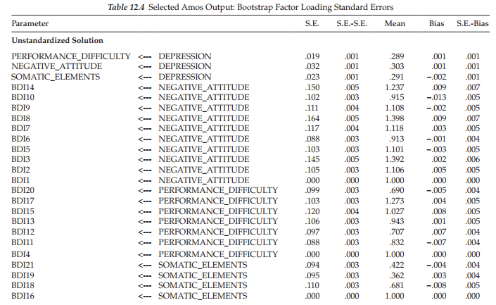
Before turning to the bootstrap results related to our Swedish sample, I need first to explain how to obtain this information from the output tree as it is not exactly a straightforward retrieval process. That is, just clicking on the Estimates label listed in the bootstrap section will yield nothing. A breakdown of the needed output is captured in Figure 12.6. To initiate the process, double-click on Estimates in the upper ML section of the tree, which yields the “Scalars” label. Double-clicking on Scalars then produces the five categories of estimates shown in Figure 12.6. It is imperative that you click on one of these five types of estimates, which will highlight the one of interest; regression weights are highlighted in the figure, although the highlighting is rather faded. Once you have identified the estimates of interest (in this case, the regression weights), the bootstrap section then becomes activated. Clicking on the “bootstrap standard errors” resulted in the standard error information presented in Table 12.4.

The first column (S.E.) in the table lists the bootstrap estimate of the standard error for each factor loading parameter in the model. This value represents the standard deviation of the parameter estimates computed across the 500 bootstrap samples. These values should be compared with the approximate ML standard error estimates presented in Table 12.3. In doing so, you will note several large discrepancies between the two sets of standard error estimates. For example, in a comparison of the stand­ard error for the loading of BDI Item 9 (BDI9) on the Negative Attitude factor across the original (S.E. = .057) and bootstrap (S.E. = .111) samples, we see a differential of 0.054, which represents a 95% increase in the boot­strap standard error over that of the ML error. Likewise, the bootstrap standard error for the loading of Item 3 (BDI3) on the same factor is 99% larger than the ML estimate (.145 vs. .073). These findings suggest that the distribution of these parameter estimates appear to be wider than would be expected under normal theory assumptions. No doubt, these results reflect the presence of outliers, as well as the extremely kurtotic nature of these data.

The second column, labeled “S.E.-S.E.”, provides the approximate standard error of the bootstrap standard error itself. As you will see, these values are all very small, and so they should be. Column 3, labeled “Mean”, lists the average parameter estimate computed across the 500 bootstrap samples. It is important to note that this bootstrap mean is not necessarily identical to the original estimate and, in fact, it can often be quite differ­ent (Arbuckle & Wothke, 1999). The information provided in Column 4 (“Bias”) represents the difference between the original estimate and the mean of estimates across the bootstrap samples. In the event that the mean estimate of the bootstrap samples is higher than the original estimate, then the resulting bias will be positive. Finally, the last column, labeled “S.E.- Bias”, reports the approximate standard error of the bias estimate.

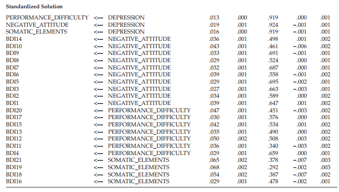
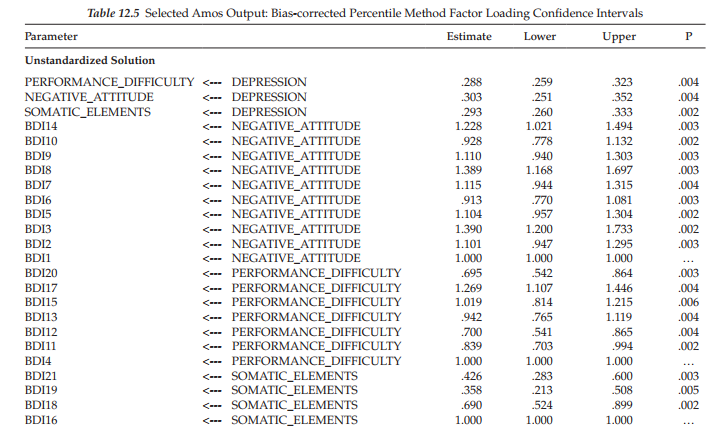
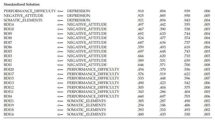
Bootstrap bias-corrected confidence intervals. The last set of information to be presented here relates to the 90% (default) bias-corrected confidence intervals for both the unstandardized and standardized factor loading estimates, which are reported in Table 12.5. Although Amos has the capa­bility to produce percentile, as well as bias-corrected confidence inter­vals, the latter are considered to yield the more accurate values (Efron & Tibshirani, 1993). Values for BDI items 1, 4, and 16 are replaced with dots (…) as these parameters were constrained to a nonzero value for purposes of model identification. Bias-corrected confidence intervals are interpreted in the usual manner. For example, the loading of BDI14 on the factor of Negative Attitude has a confidence interval ranging from 1.021 to 1.494. Because this range does not include zero, the hypothesis that the BDI14 factor loading is equal to zero in the population can be rejected. This infor­mation can also be derived from the p values which indicate how small the confidence level must be to yield a confidence interval that would include zero. Turning again to the BDI14 parameter, then, a p-value of .003 implies that the confidence interval would have to be at the 99.7% level before the lower bound value would be zero.

Finally, I wish to briefly introduce you to the Bollen-Stine bootstrap­ping option, an approach developed by Bollen and Stine (1993) to improve upon the usual nonparametric procedure described thus far in this chapter. They noted that although this general bootstrapping procedure can work well in many cases, it can also fail. Bollen and Stine (1993, p. 113) pointed out that “The success of the bootstrap depends on the sampling behavior of a statistic being the same when the samples are drawn from the empir­ical distribution and when they are taken from the original population.” In other words, the statistical values should be the same when based on the original population and on the initial (i.e., parent) sample from which the bootstrapped samples are drawn. Although this assumption under­lies the bootstrapping process, Bollen and Stine contend that this assump­tion does not always hold and, as a result, the bootstrap samples perform poorly.

In an attempt to address this problem, Bollen and Stine (1993) pro­posed that the parent sample data be transformed such that its covariance matrix is equivalent to the model-implied covariance matrix with the aim of having a perfect model fit. As such, the transformed data would then have the same distributional characteristics as the original parent sample but represent the null condition of a perfectly fitting model (Hancock & Liu, 2012). Each bootstrap sample is then drawn from this transformed data set and a chi-square value computed for the fit of that bootstrapped data to the model. These chi-square values are compared internally to the chi-square value that was computed for the initial observed data fitted to the model (reported in the Notes for Model section of output). The pro­portion of times the model “fit worse” (i.e., the number of times that the model chi-square for the bootstrapped sample exceeded the chi-square for the observed data) represents the Bollen-Stine bootstrap p-value.

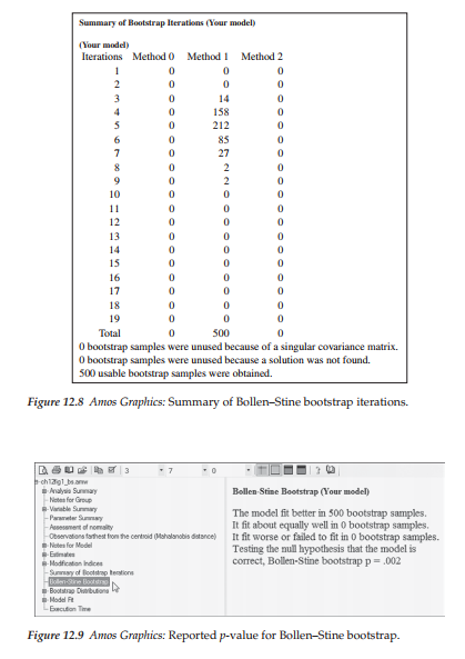
To give you a snapshot view of bootstrap results based on the Bollen-Stine bootstrapping approach, I reran the hypothesized model (Figure 12.1), but in contrast to the previous nonparametric approach based on ML bootstrapping, I selected the Bollen-Stine option in the Analysis Properties dialog box (for a review of this box, see Figure 12.2). Resulting output related to a request for the Bollen-Stine bootstrapping approach is presented in three separate sections. The first section presents the same type of summary diagnostics as shown earlier for the nonpara­metric approach and is shown in Figure 12.8. In comparing this summary with the one for the nonparametric procedure (see Figure 12.7), we see that although all 500 samples were used and obtained in 19 iterations for both, the coordinates between the number of bootstrap samples and the number of iterations taken to complete this sampling process varied. For example, let’s once again compare the information presented on line 4 of this summary report. Whereas the minimum was achieved in 4 itera­tions for only 65 bootstrap samples for the nonparametric approach, 158 bootstrap samples were obtained in the same number of iterations for the Bollen-Stine approach.

The second set of output information states that the model fit better in 500 bootstrap samples and worse in 0 bootstrap samples with a reported p-value of .002 (see Figure 12.9). When bootstrapping is used in address­ing the issue of multivariate nonnormal data, it is this p-value that should be used in place of the original model ML p-value. However, as is well known in the SEM literature and as you will also readily recognize by now, the chi-square value for the hypothesized model, particularly when the sample size is large, will typically always suggest rejection of the model. Thus, it is not surprising that this p-value is <.05. Nonetheless, given that the ML p-value was .000, the Bollen-Stine p-value represents at least some improvement in this respect. A review of the goodness-of- fit indices for this model reveal the CFI value to be .91 for this model, indicating that it represents only a marginally well-fitting model at best.

However, as described earlier, this model was extrapolated from a study in which models of the BDI were tested for their multigroup invariance. Given that use of this model was intended solely to illustrate the basic pro­cedures involved in conducting a bootstrapping analysis in Amos, it had not been subjected to any post hoc modifications. However, for readers intending to use these bootstrap procedures for the purpose of address­ing nonnormality data issues, I strongly advise you to first determine the most parsimonious yet best-fitting model prior to applying the bootstrap procedures.

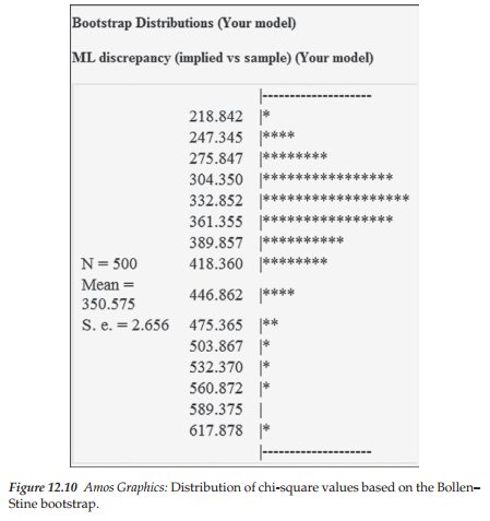
Finally, the third section of the Bollen-Stine bootstrap output displays the distribution of chi-square values obtained for the 500 bootstrap sam­ples as shown in Figure 12.10. The most noteworthy features of this output information are the mean chi-square value (350.575) and the overall shape of this distribution, which is clearly nonnormal.

In this chapter, I have endeavored to give you a flavor of how Amos enables you to conduct the bootstrap procedure. Due to space limita­tions, I have not been able to include details or examples related to the use of bootstrapping for comparisons of models and/or estimation meth­ods. However, for readers who may have an interest in these types of applications, this information is well presented in the Amos User’s Guide (Arbuckle, 2015).

Source: Byrne Barbara M. (2016), Structural Equation Modeling with Amos: Basic Concepts, Applications, and Programming, Routledge; 3rd edition.