Application 8: Testing Evidence of Construct Validity with AMOS: The Multitrait-Multimethod Model

1. Key Concepts

• The dual focus of construct validation procedures
• Convergent validity, discriminant validity, and method effects
• Reorientation of Amos Graphics models to fit page size
• Comparison of the correlated traits-correlated methods (CT-CM) and correlated traits-correlated uniquenesses (CT-CU) multitrait- multimethod models
• Warning messages regarding inadmissible solutions and negative variances

Construct validity embraces two modes of inquiry: (a) validation of a con­struct (or trait) and (b) validation of a measuring instrument. In valid­ating a construct, the researcher seeks empirical evidence in support of hypothesized relations among dimensions of the same construct (termed within-network relations), and among the construct of interest and other dissimilar constructs (termed between-network relations). Both theoret­ical linkages represent what Cronbach and Meehl (1955) referred to as representing the construct’s nomological network. Validation of a meas­uring instrument, on the other hand, requires empirical evidence that the scale items do, in fact, measure the construct of interest and, in the case of a multidimensional construct, that the related subscales exhibit a well-defined factor structure that is consistent with the underlying theory.

The application illustrated in this chapter focuses on the latter. Specifically, CFA procedures within the framework of a multitrait- multimethod (MTMM) design are used to test hypotheses bearing on the construct validity of an assessment scale. Accordingly, multiple traits are measured by multiple methods. Following from the seminal work of Campbell and Fiske (1959), construct validity research pertinent to a meas­uring instrument typically focuses on the extent to which data exhibit evi­dence of: (a) convergent validity, the extent to which different assessment methods concur in their measurement of the same trait; ideally, these values should be moderately high, (b) discriminant validity, the extent to which independent assessment methods diverge in their measurement of different traits; ideally, these values should demonstrate minimal con­vergence, and (c) method effects, an extension of the discriminant validity issue. Method effects represent bias that can derive from use of the same method in the assessment of different traits; correlations among these traits are typically higher than those measured by different methods.

For over 50 years now (Eid & Nussbeck, 2009), the multitrait-multimethod (MTMM) matrix has been a favored methodological strategy in testing for evidence of construct validity. During this time span, however, the ori­ginal MTMM design (Campbell & Fiske, 1959) has been the target of much criticism as methodologists have uncovered a growing number of limita­tions in its basic analytic strategy (see, e.g., Bagozzi & Yi, 1993; Marsh, 1988, 1989; Schmitt & Stults, 1986). Although several alternative MTMM approaches have been proposed in the interim, the analysis of MTMM data within the framework of CFA models has gained the most promin­ence. The MTMM models of greatest interest within this analytic context include the correlated trait-correlated method (CT-CM) model (Widaman, 1985), the correlated uniquenesses (CT-CU) model (Kenny, 1979; Marsh, 1988, 1989), the composite direct product (CDP) model (Browne, 1984b), and the more recent correlated trait-correlated methods minus one (CT-C[M-1]) model (Eid, 2000). Although some researchers argue for the superior­ity of the CT-CU model (e.g., Kenny, 1976, 1979; Kenny & Kashy, 1992; Marsh, 1989; Zhang, Jin, Leite, & Algina, 2014), others support the CT-CM model (e.g., Conway, Scullen, Lievens, & Lance, 2004; Lance, Noble, & Scullen, 2002). Nonetheless, a review of the applied MTMM literature reveals that the CT-CM model has been and continues to be the method of choice, albeit with increasingly more and varied specifications of this model (see, e.g., Eid et al., 2008; Hox & Kleiboer, 2007; LaGrange & Cole, 2008). The popularity of this approach likely derives from Widaman’s (1985) seminal paper in which he proposed a taxonomy of nested model comparisons. (For diverse comparisons of the CT-CM, CT-CU, CDP, and CT-C[M-1] models, readers are referred to Bagozzi, 1993; Bagozzi & Yi, 1990, 1993; Byrne & Goffin, 1993; Castro-Schilo, Widaman, & Grimm, 2013; Castro-Schilo, Widaman, & Grimm, 2014; Coenders & Saris, 2000; Geiser, Koch, & Eid, 2014; Hernandez & Gonzalez-Roma, 2002; Lance et al., 2002; Marsh & Bailey, 1991; Marsh, Byrne, & Craven, 1992; Marsh & Grayson, 1995; Tomas, Hontangas, & Oliver, 2000; Wothke, 1996; Zhang et al., 2014.)

Although method effects have also been of substantial interest in all MTMM models during this same 50-year period, several researchers (e.g., Cronbach, 1995; Millsap, 1995; Sechrest, Davis, Stickle, & McKnight, 2000) have called for a more specific explanation of what is meant by the term “method effects” and how these effects are manifested in different MTMM models. Geiser, Eid, West, Lischetzke, and Nussbeck (2012) recently addressed this concern through a comparison of two MTMM modeling approaches in which they introduced the concepts of individual, condi­tional, and general method bias and showed how these biases were repre­sented in each model.

The present application is taken from a study by Byrne and Bazana (1996) that was based on the CT-CM approach to MTMM analysis. However, given increasing interest in the CT-CU model over the inter­vening years, I also work through an analysis based on this approach to MTMM data. The primary intent of the original study was to test for evi­dence of convergent validity, discriminant validity, and method effects related to four facets of perceived competence (social, academic, English, mathematics) as measured by self, teacher, parent, and peer ratings for early and late preadolescents and adolescents in grades 3, 7, and 11, respectively. For our purposes here, however, we focus only on data for late preadolescents (grade 7; n = 193). (For further elaboration of the sam­ple, instrumentation, and analytic strategy, see Byrne & Bazana, 1996.)

Rephrased within the context of a MTMM design, the model of interest in this chapter is composed of four traits (Social Competence, Academic Competence, English Competence, Mathematics Competence), and four methods (Self-ratings, Teacher Ratings, Parent Ratings, Peer Ratings). A schematic portrayal of this model is presented in Figure 10.1.

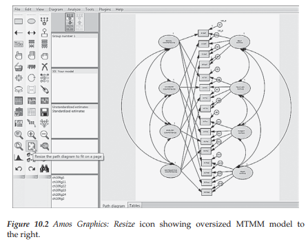
Before launching into a discussion of this model, I consider it worth­while to take a slight diversion in order to show you an option in the Amos toolbar that can be very helpful when you are working with a com­plex model that occupies a lot of page space such as we have here. The difficulty with the building of this model is that the double-headed arrows extend beyond the drawing space allotted by the program. In Figure 10.2, however, I illustrate how you can get around that problem simply by clicking on the Resize icon identified with the cursor as shown to the left of the model. Clicking on this tool will immediately resize the model to fit within the page perimeter.

2. The Correlated Traits-Correlated Methods Approach to MTMM Analyses

In testing for evidence of construct validity within the framework of the CT-CM model, it has become customary to follow guidelines set forth by Widaman (1985). As such, the hypothesized MTMM model is compared with a nested series of more restrictive models in which specific parameters are either eliminated, or constrained equal to zero or 1.0. The difference in X² (Ax²) provides the yardstick by which to judge evidence of convergent and discriminant validity. Although these evaluative comparisons are made solely at the matrix level, the CFA format allows for an assessment of construct validity at the individual parameter level. A review of the literature bearing on the CFA approach to MTMM analyses indicates that assessment is typically formulated at both the matrix and the individual parameter levels; we examine both in the present application.

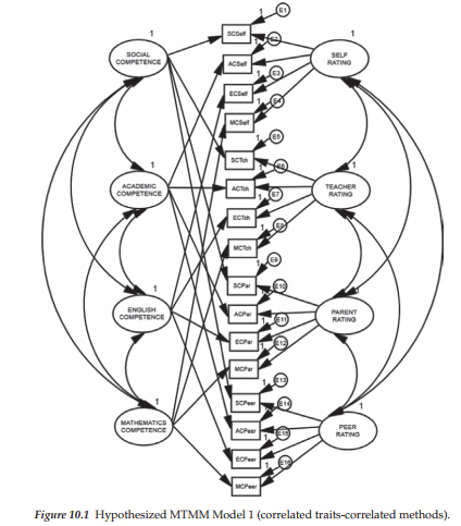
The MTMM model portrayed in Figure 10.1 represents the hypothe­sized model and serves as the baseline against which all other alternatively nested models are compared in the process of assessing evidence of construct and discriminant validity. Clearly, this CFA model represents a much more complex structure than any of the CFA models examined thus far in this book. This complexity arises primarily from the loading of each observed variable onto both a trait and a method factor. In addition, the model postulates that, although the traits are correlated among them­selves, as are the methods, any correlations between traits and methods are assumed to be zero.¹

Testing for evidence of construct and discriminant validity involves comparisons between the hypothesized model (Model 1) and three alter­native MTMM models. We turn now to a description of these four nested models; they represent those most commonly included in CFA MTMM analyses.

Model 1: Correlated Traits-Correlated Methods

The first model to be tested (Model 1) represents the hypothesized model shown in Figure 10.1 and serves as the baseline against which all alternative MTMM models are compared. As noted earlier, because its specification includes both trait and method factors, and allows for correlations among traits and among methods, this model is typically the least restrictive.²

Before working through the related analyses, I wish first to clarify the names of the variables, and then to point out two important and unique features regarding the specification of factor variances and covariances related to this first model. With respect to the labeling mechanism, the var­iables SCSelf to SCPeer represent general Social Competence (SC) scores as derived from self, teacher, parent, and peer ratings. Relatedly, for each of the remaining traits (Academic SC, English SC, Math SC) there are rat­ings by self, teacher, parents, and peers.

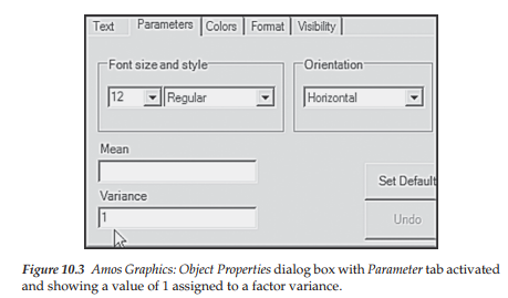
We turn now to the two critically important features of this model. First, in viewing Figure 10.1, you will see a “1” above each of the six fac­tors in the model. This specification indicates that the variance for each of these factors is fixed to 1.00. The question now is: Why are these factor variances specified as fixed parameters in the model? In answering this question, recall from Chapter 5 that in the specification of model param­eters one can either estimate a factor loading or estimate the variance of its related factor, but one cannot estimate both; the rationale underlying this caveat is linked to the issue of model identification. In all previous examples thus far in the book, one factor loading in every set of congen­eric measures has been fixed to 1.00 for this purpose. However, in MTMM models, interest focuses on the factor loadings and, thus, this alternative approach to model identification is implemented. The process of fixing the factor variance to a value of 1.0 is easily accomplished in Amos Graphics by first right-clicking on the factor, selecting Object Properties, clicking on the Parameter tab, and then entering a “1” in the Variance box as shown in Figure 10.3.

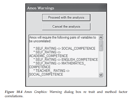
Second, note in Figure 10.1 that all trait (Social Competence to Mathematics Competence) and method (Self-Rating to Peer Rating) covar­iances are freely estimated. Importantly, however, you will see that covari­ances among traits and methods have not been specified (see Note 1). Let’s turn now to the test of this correlated traits-correlated methods (CT-CM) model. Immediately upon clicking on the Calculate icon (or drop-down menu), you will be presented with the dialog box shown in Figure 10.4, which lists a series of covariance parameters and warns that these pairs must remain uncorrelated. In fact, the parameters listed represent all covariances between trait and method factors, which I noted earlier in this chapter cannot be estimated for statistical reasons. Thus we can proceed by clicking on the Proceed with the Analysis tab.³

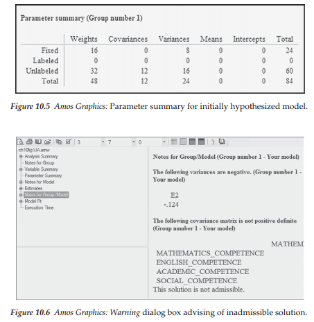
In reviewing results for this initial analysis we turn first to the “Parameter summary” table, which is shown in Figure 10.5. Listed first in this summary are 48 weights (i.e., regression paths): 16 fixed weights asso­ciated with the error terms and 32 estimated weights associated with the factor loadings. Next, we have 12 covariances (6 for each set of trait and method factors) and 24 variances (8 fixed factor variances; 16 estimated error variances).

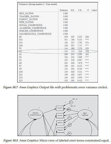
The next critically important result reported in the output file is an alert message in the “Notes for Group/Model” file as shown in Figure 10.6. This message advises that the variance of error term E2 is negative, thereby result­ing in a covariance matrix that is not positive definite, and at the bottom that the solution is not admissible. Indeed, a review of the estimates for this solu­tion confirms that the variance associated with the error term E2 is negative.

It is now widely known that the estimation of improper estimates, such as these, is a common occurrence with applications of the CT-CM model to MTMM data. Indeed, so pervasive is this problem, that the estimation of a proper solution may be regarded as a rare find (see, e.g., Kenny & Kashy, 1992; Marsh, 1989). Although these results can be triggered by a number
of factors, one likely cause in the case of MTMM models is the overparam­eterization of the model (see Wothke, 1993); this condition likely occurs as a function of the complexity of specification. In addressing this con­undrum, early research has suggested a reparameterization of the model in the format of the correlated uniqueness (CU) model (see Kenny, 1976, 1979; Kenny & Kashy, 1992; Marsh, 1989; Marsh & Bailey, 1991; Marsh & Grayson, 1995). Alternative approaches have appeared in the more recent literature; these include the use of multiple indicators (Eid, Lischetzke, Nussbeck, & Trierweiler, 2003; Tomas, Hontangas, & Oliver, 2000), the specification of different models for different types of methods (Eid et al., 2008), and the specification of equality constraints in the CT-CU model (Coenders & Saris, 2000; Corten et al., 2002). Because the CT-CU model has become the topic of considerable interest and debate over the past few years, I considered it worthwhile to include this model also in the present chapter. However, given that (a) the CT-CU model represents a special case of, rather than a nested model within the CT-CM framework, and (b) it is important first to work through the nested model comparisons proposed by Widaman (1985), I delay discussion and application of this model until later in the chapter.

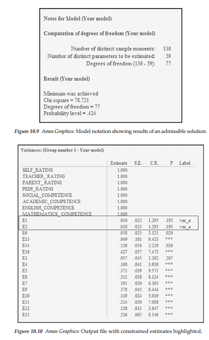
Returning to our inadmissible solution, let’s review the variance esti­mates (shown in Figure 10.7) where we find a negative variance associated with error term E2. Important to this result is a study by Marsh, Byrne, and Craven (1992) showing that when improper solutions occur in CFA modeling of MTMM data, one approach to resolution of the problem is to impose an equality constraint between parameters having similar esti­mates. Thus, in an attempt to resolve the inadmissible solution problem, Model 1 was respecified with the error variance for E2 constrained equal to that for E1, which represented a positive value of approximately the same size. Assignment of this constraint was implemented via the Amos labeling process illustrated and captured in Figure 10.8. (For a review of this process see Chapters 5 and 7.)

This respecified model yielded a proper solution, the summary of which is reported in Figure 10.9; the estimates pertinent to the variances only are reported in Figure 10.10. As can be see from the latter, this minor respecification resolved the negative error variance, resulting in both parameters having an estimated value of .030.

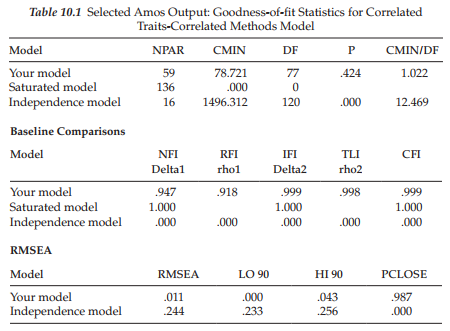
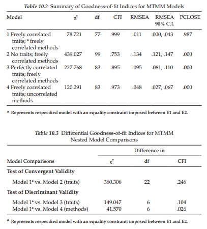
Goodness-of-fit statistics related to this model are reported in Table 10.1. As evidenced from these results, the fit between this respecified CT-CM model and the data was almost perfect (CFI = .999; RMSEA = .011; 90% C.I. .000, .043). Indeed, had additional parameters been added to the model as a result of post hoc analyses, I would have concluded that the results were indicative of an overfitted model. However, because this was not the case, I can only presume that the model fits the data exceptionally well.

We turn now to three additional MTMM models against which modi­fied Model 1 will be compared.

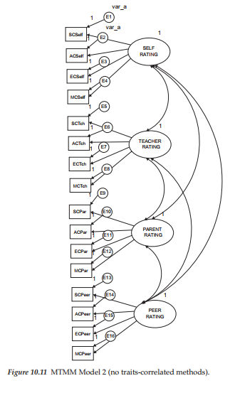
Model 2: No Traits-Correlated Methods

Specification of parameters for this model is portrayed schematically in Figure 10.11. Of major importance with this model is the total absence of trait factors. It is important to note that for purposes of comparison across all four MTMM models, the constraint of equality between the error terms E1 and E2 is maintained throughout. Goodness-of-fit for this model proved to be very poor (x²₍₉₉₎ = 439.027; CFI = .753; RMSEA = .134, 90% C.I. .121, .147). A sum­mary of comparisons between this model and Model 1, as well as between all remaining models, is tabulated following this review of each MTMM model.

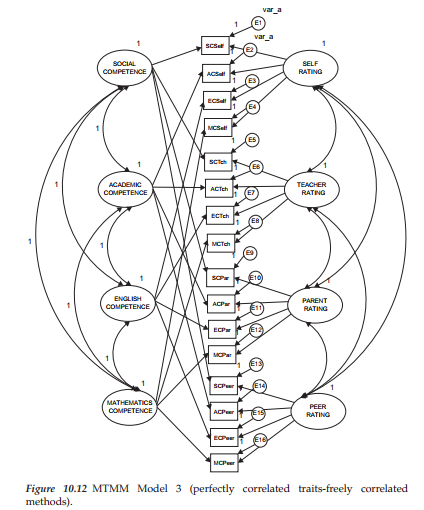
Model 3: Perfectly Correlated Traits-Freely Correlated Methods

In reviewing the specification for Model 3 shown in Figure 10.12, we can see that as with the hypothesized CT-CM model (Model 1), each observed variable loads on both a trait and a method factor. However, in stark con­trast to Model 1, this MTMM model argues for trait correlations that are perfect (i.e., they are equal to 1.0); consistent with both Models 1 and 2, the method factors are freely estimated. Although goodness-of-fit results for this model were substantially better than for Model 2, they nonethe­less were indicative of only a marginally well-fitting model and one that was somewhat less well-fitting than Model 1 (x²(₈₃) = 227.768; CFI = .895; RMSEA = .011, 90% C.I. .081, .110).

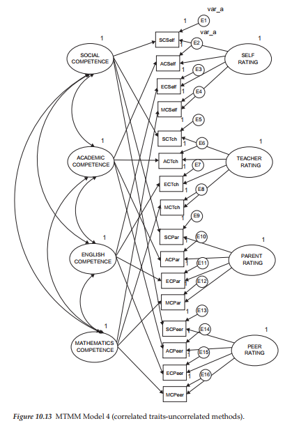
Model 4: Freely Correlated Traits-Uncorrelated Methods

This final MTMM model is portrayed in Figure 10.13 and differs from Model 1 only in the absence of specified correlations among the method factors. Goodness-of-fit results for this model revealed an exception­ally good fit to the data (x²₍₈₃₎ = 120.291; CFI = .973; RMSEA = .048, 90% C.I .= .027, .067).

3. Testing for Evidence of Convergent and Discriminant Validity: MTMM Matrix-level Analyses

Comparison of Models

Now that we have examined goodness-of-fit results for each of the MTMM models, we can turn to the task of determining evidence of construct and discriminant validity, as well as method effects. In this section, we ascer­tain information at the matrix level only, through the comparison of par­ticular pairs of models. A summary of goodness-of-fit results related to all four MTMM models is presented in Table 10.2, and results of model comparisons are summarized in Table 10.3.

Evidence of Convergent Validity

As noted earlier, one criterion of construct validity bears on the issue of convergent validity, the extent to which independent measures of the same trait are correlated (e.g., teacher ratings and self-ratings of social com­petence); these values should be substantial and statistically significant (Campbell & Fiske, 1959). Using Widaman’s (1985) paradigm, evidence of convergent validity can be tested by comparing a model in which traits are specified (Model 1), with one in which they are not (Model 2), the difference in x² between the two models (Ax²) providing the basis for judgment; a significant difference in x² supports evidence of convergent validity. In an effort to provide indicators of nested model comparisons that were more realistic than those based on the x² statistic, Bagozzi and Yi (1990), Widaman (1985), and others, have examined differences in CFI values. However, until the work of Cheung and Rensvold (2002), these ACFI values have served in only a heuristic sense as an evaluative base upon which to determine evidence of convergent and discriminant valid­ity. Recently, Cheung and Rensvold (2002) examined the properties of 20 goodness-of-fit indices, within the context of invariance testing and arbi­trarily recommended that ACFI values should not exceed .01. Although the present application does not include tests for invariance, the same principle holds regarding the model comparisons. As shown in Table 10.3, the Ax² was highly significant (x²(₂₂) = 360.306, p < .001), and the difference in practical fit (ACFI = .246) substantial, thereby arguing for the tenability of this criterion.

Evidence of Discriminant Validity

Discriminant validity is typically assessed in terms of both traits, and methods. In testing for evidence of trait discriminant validity, one is interested in the extent to which independent measures of different traits are correlated; these values should be negligible. When the independent measures represent different methods, correlations bear on the discrimin­ant validity of traits; when they represent the same method, correlations bear on the presence of method effects, another aspect of discriminant validity.

In testing for evidence of discriminant validity among traits, we compare a model in which traits correlate freely (Model 1), with one in which they are perfectly correlated (Model 3); the larger the discrepancy between the x², and the CFI values, the stronger the support for evidence of discriminant validity. This comparison yielded a Ax² value that was statistically significant (x²(₆) = 149.047, p < .001), and the difference in prac­tical fit was fairly large (ACFI = .100, suggesting only modest evidence of discriminant validity. As was noted for the traits (Note 3), we could alternatively specify a model in which perfectly correlated method fac­tors are specified; as such, a minimal Ax² would argue against evidence of discriminant validity.

Based on the same logic, albeit in reverse, evidence of discriminant validity related to method effects can be tested by comparing a model in which method factors are freely correlated (Model 1) with one in which the method factors are specified as uncorrelated (Model 4). In this case, a large Ax² (or substantial ACFI) argues for the lack of discriminant validity and, thus, for common method bias across methods of measurement. On the strength of both statistical (Ax²(₆) = 41.570) and nonstatistical (ACFI = .026) criteria, as shown in Table 10.3, it seems reasonable to conclude that evi­dence of discriminant validity for the methods was substantially stronger than it was for the traits.

4. Testing for Evidence of Convergent and Discriminant Validity: MTMM Parameter-level Analyses

Examination of Parameters

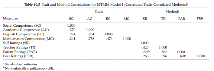
A more precise assessment of trait- and method-related variance can be ascertained by examining individual parameter estimates. Specifically, the factor loadings and factor correlations of the hypothesized model (Model 1) provide the focus here. Because it is difficult to envision the MTMM pattern of factor loadings and correlations from the output when more than six factors are involved, these values have been tabled to facilitate the assessment of convergent and discriminant validity; standardized estimates for the factor loadings are summarized in Table 10.4 and for the factor correlations in Table 10.5. (For a more extensive discussion of these MTMM findings, see Byrne & Bazana, 1996.)

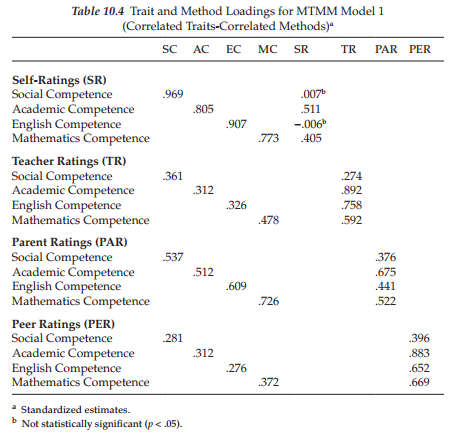
Evidence of Convergent Validity

In examining individual parameters, convergent validity is reflected in the magnitude of the trait loadings. As indicated in Table 10.4, all trait loadings are statistically significant with magnitudes ranging from .276 (peer ratings of English Competence) to .969 (self-ratings of Social Competence). However, in a comparison of factor loadings across traits and methods, we see that the proportion of method variance exceeds that of trait variance for all but one of the teacher ratings (Social Competence), only one of the parent ratings (Academic Competence) and all of the peer ratings.⁴ Thus although, at first blush, evidence of convergent val­idity appeared to be fairly good at the matrix level, more in-depth exam­ination at the individual parameter level reveals the attenuation of traits by method effects related to teacher and peer ratings, thereby temper­ing evidence of convergent validity (see also, Byrne & Goffin, 1993 with respect to adolescents).

Evidence of Discriminant Validity

Discriminant validity bearing on particular traits and methods is deter­mined by examining the factor correlation matrices. Although, concep­tually, correlations among traits should be negligible in order to satisfy evidence of discriminant validity, such findings are highly unlikely in gen­eral, and with respect to psychological data in particular. Although these findings, as shown in Table 10.5, suggest that relations between perceived academic competence (AC), and the subject-specific perceived competen­cies of English (EC) and mathematics (MC), are most detrimental to the attainment of trait discriminant validity, they are nonetheless consistent with construct validity research in this area as it relates to late preadoles­cent children (see Byrne & Worth Gavin, 1996).

Finally, an examination of method factor correlations in Table 10.5 reflects on their discriminability, and thus on the extent to which the methods are maximally dissimilar; this factor is an important underlying assumption of the MTMM strategy (see Campbell & Fiske, 1959). Given the obvious dissimilarity of self, teacher, parent, and peer ratings, it is somewhat surprising to find a correlation of .562 between teacher and par­ent ratings of competence. One possible explanation of this finding is that, except for minor editorial changes necessary in tailoring the instrument to either teacher or parent as respondents, the substantive content of all comparable items in the teacher and parent rating scales were identically worded; the rationale here being to maximize responses by different raters of the same student.

5. The Correlated Uniquenesses Approach to MTMM Analyses

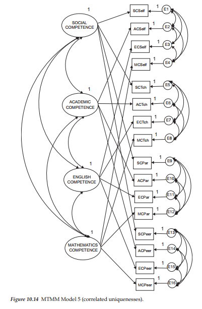
As noted earlier, the CT-CU model represents a special case of the CT-CM model. Building upon the early work of Kenny (1976, 1979), Marsh (1988, 1989) proposed this alternative MTMM model in answer to the numerous estimation and convergence problems encountered with analyses of the CT-CM model. Recently, however, research has shown that the CT-CU model also is not without its own problems, for which researchers have proposed a number of specification alternatives (see, e.g., Conway et al., 2004; Lance et al., 2002; Corten et al., 2002). The hypothesized CT-CU model tested here, however, is based on the ori­ginally postulated CT-CU model (see, e.g., Kenny, 1976, 1979; Kenny & Kashy, 1992; Marsh, 1989). A schematic representation of this model is shown in Figure 10.14.

In reviewing the model depicted in Figure 10.14, you will note that it embodies only the four correlated trait factors; in this aspect only, it is consistent with the CT-CM model shown in Figure 10.1. The notably different feature about the CT-CU model, however, is that although no method factors are specified per se, their effects are implied from the specification of correlated error terms (the uniquenesses)⁵ associated with each set of observed variables embracing the same method. For example, as indicated in Figure 10.14, all error terms associated with the self-rating measures of Social Competence are correlated with one another. Likewise, those associated with teacher, parent, and peer rat­ings are intercorrelated.

Consistent with the correlated traits-uncorrelated methods model (Model 4 in this application), the CT-CU model assumes that effects asso­ciated with one method, are uncorrelated with those associated with the other methods (Marsh & Grayson, 1995). However, one critically important difference between the CT-CU model, and both the correlated traits-correlated methods (Model 1) and Correlated Traits/No Methods (Model 4) models involves the assumed unidimensionality of the method factors. Whereas Models 1 and 4 implicitly assume that the method effects associated with a particular method are unidimensional (i.e., they can be explained by a single latent method factor), the CT-CU model car­ries no such assumption (Marsh & Grayson, 1995). These authors fur­ther note (p. 185) that when an MTMM model includes more than three trait factors, this important distinction can be tested. However, when the number of traits equals three, the CT-CU model is formally equivalent to the other two in the sense that the “number of estimated parameters and goodness-of-fit are the same, and parameter estimates from one can be transformed into the other.”

Of course, from a practical perspective, the most important distinc­tion between the CT-CU model and Models 1 and 4, is that it typically results in a proper solution (Kenny & Kashy, 1992; Marsh, 1989; Marsh & Bailey, 1991). Model 1, on the other hand, is now notorious for its ten­dency to yield inadmissible solutions, as we observed in the present appli­cation. As a case in point, Marsh and Bailey (1991), in their analyses of 435 MTMM matrices based on both real and simulated data, reported that, whereas the CT-CM model resulted in improper solutions 77% of the time, the CT-CU model yielded proper solutions nearly every time (98%). (For additional examples of the incidence of improper solutions with respect to Model 1, see Kenny & Kashy, 1992). We turn now to the analyses based on the CT-CU model (Model 5).

Model 5: Correlated Uniquenesses Model

Reviewing, once again, the model depicted in Figure 10.14, we see that there are only four trait factors, and that these factors are hypothesized to correlate among themselves. In addition, we find the correlated error terms associated with each set of observed variables derived from the same measuring instrument (i.e., sharing the same method of measurement).

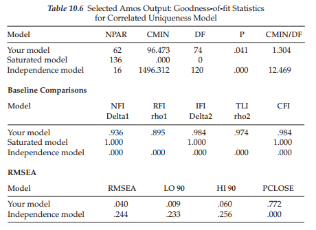
We turn now to selected sections of the Amos output file pertinent to this correlated uniquenesses model. In reviewing Table 10.6, we see that this model represents an excellent fit to the data (x²(₇₄) = 96.473; CFI = .984; RMSEA = .040, 90% C.I. = .009, .060). Furthermore, consistent with past reported results (e.g., Kenny & Kashy, 1992; Marsh & Bailey, 1991), this solution resulted in no problematic parameter estimates.

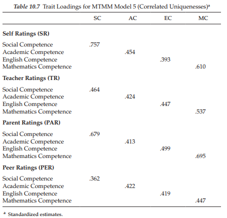
Assessment of convergent and discriminant validity related to the CT-CU model can be accomplished in the same way as it is for the CT-CM model when focused at the individual parameter level. As can be seen in Table 10.7, evidence related to the convergent validity of the traits, not surprisingly, was substantial. Although all parameters were similar in terms of substantiality to those presented for Model 1 (see Table 10.4), there are interesting differences between the two models. In particular, these differences reveal all teacher and peer rating loadings to be higher for the CT-CU model than for Model 1. Likewise, parent ratings, as they relate only to Social Competence, are also higher than for Model 1.

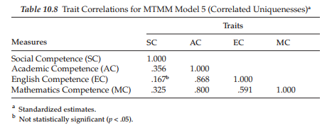
Let’s look now at the factor correlations relevant to the traits; these estimates are presented in Table 10.8. In reviewing these values, we see that all but one estimated value are statistically significant and, for the most part, of similar magnitude across Model 1 and the CT-CU model. The correlation between Social Competence and English Competence was found not to be statistically significant (p < .05) for the CT-CU model.

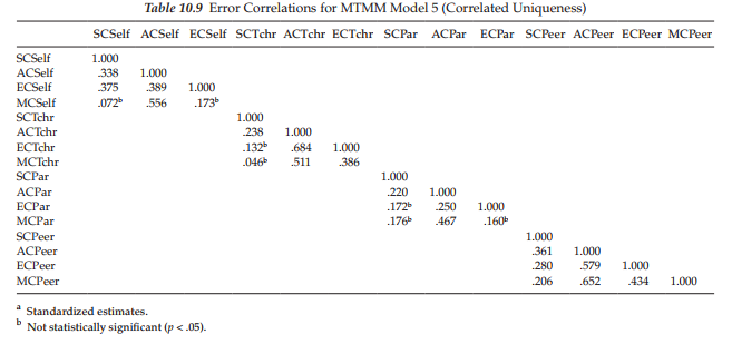
Method effects in the CT-CU model are determined by the degree to which the error terms are correlated with one another (Kenny & Kashy, 1992). In contrast to Model 1, there is no assumption that the method factor remains the same for all measures embracing the same method. Rather, as Kenny and Kashy (1992, p. 169) explain, “In the Correlated Uniquenesses model, each measure is assumed to have its own method effect, and the covariances between measures using the same method assess the extent to which there is a common method factor.” In other words, as Kenny and Kashy further note, whereas the general CFA MTMM model assumes that method effects are invariant across traits, the CT-CU model allows for the multidimensionality of method effects. (For critiques of these effects, see Conway et al., 2004; Lance et al., 2002; for an attempt to understand the substance of these correlated error terms, see Saris & Aalberts, 2003.) It is interesting to see in Table 10.9, that the strongest method effects are clearly associated with teacher and peer ratings of the three academic competen­cies, and with parent ratings of only Mathematics Competence. Indeed, from a substantive standpoint, these findings at least for the teacher and peer ratings certainly seem perfectly reasonable. On the other hand, the strong method effects shown for parent ratings involving relations between academic and math competencies is intriguing. One possible explanation may lie in the fact that when parents think “academic compe­tence,” their thoughts gravitate to “math competence.” As such, academic competence appears to be defined in terms of how competent they per­ceive their son or daughter to be in math.

In concluding this chapter, it is worthwhile to underscore Marsh and Grayson’s (1995, p. 198) recommendation regarding the analysis of MTMM data. As they emphasize, “MTMM data have an inherently com­plicated structure that will not be fully described in all cases by any of the models or approaches typically considered. There is, apparently, no ‘right’ way to analyze MTMM data that works in all situations.” Consequently, Marsh and Grayson (1995), supported by Cudeck (1988), strongly advise that in the study of MTMM data, researchers should always consider alternative modeling strategies (see, e.g., Eid et al., 2008). In particular, Marsh and Grayson (1995) suggest an initial examination of data within the framework of the original Campbell-Fiske guidelines. This analysis should then be followed by the testing of a subset of at least four CFA models (including the CT-CU model); for example, the five models con­sidered in the present application would constitute an appropriate sub­set. Finally, given that the composite direct product model⁶ is designed to test for the presence of multiplicative, rather than additive effects, it should also be included in the MTMM analysis alternative approach strat­egy. Indeed, Zhang et al. (2014) recently found the CT-CU model to be quite robust to multiplicative effects when the MTMM matrix included three traits and three methods. (But, for a critique of this CT-CU approach, readers are referred to Corten et al., 2002.) In evaluating results from each of the covariance structure models noted here, Marsh and Grayson (1995) caution that, in addition to technical considerations such as convergence to proper solutions and goodness-of-fit, researchers should place a heavy emphasis on substantive interpretations and theoretical framework.

Source: Byrne Barbara M. (2016), Structural Equation Modeling with Amos: Basic Concepts, Applications, and Programming, Routledge; 3rd edition.