Multiple Regression Approach to Experimental Design

In Section 15.7 we discussed the use of dummy variables in multiple regression analysis. In this section we show how the use of dummy variables in a multiple regression equation can provide another approach to solving experimental design problems. We will demonstrate the multiple regression approach to experimental design by applying it to the Chemitech, Inc., completely randomized design.

Chemitech has developed a new filtration system for municipal water supplies. The components for the new filtration system will be purchased from several suppliers, and Chemitech will assemble the components at its plant in Columbia, South Carolina. Three different assembly methods, referred to as methods A, B, and C, have been proposed. Man­agers at Chemitech want to determine which assembly method can produce the greatest number of filtration systems per week.

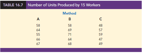
A random sample of 15 employees was selected, and each of the three assembly methods was randomly assigned to 5 employees. The number of units assembled by each employee is shown in Table 16.7. The sample mean number of units produced with each of the three assembly methods is as follows:

Although method B appears to result in higher production rates than either of the other methods, the issue is whether the three sample means observed are different enough for us to conclude that the means of the populations corresponding to the three methods of assembly are different.

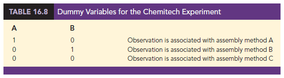
We begin the regression approach to this problem by defining dummy variables that will be used to indicate which assembly method was used. Because the Chemitech problem has three assembly methods or treatments, we need two dummy variables. In general, if the factor being investigated involves k distinct levels or treatments, we need to define k – 1 dummy variables. For the Chemitech experiment we define dummy variables A and B as shown in Table 16.8.

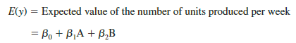
We can use the dummy variables to relate the number of units produced per week, y, to the method of assembly the employee uses.

Thus, if we are interested in the expected value of the number of units assembled per week for an employee who uses method C, our procedure for assigning numerical values to the dummy variables would result in setting A = B = 0. The multiple regression equation then reduces to

We can interpret β₀ as the expected value of the number of units assembled per week for an employee who uses method C. In other words, β₀ is the mean number of units assembled per week using method C.

Next let us consider the forms of the multiple regression equation for each of the other methods. For method A the values of the dummy variables are A = 1 and B = 0, and

For method B we set A = 0 and B = 1, and

We see that β₀ + β₁ represents the mean number of units assembled per week using method A, and β₀ + β₂ represents the mean number of units assembled per week using method B.

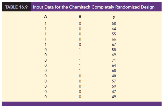
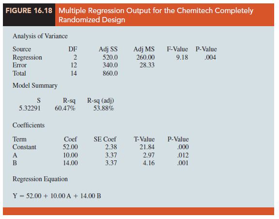
We now want to estimate the coefficients β₀, β₁, and β₂ and hence develop an estimate of the mean number of units assembled per week for each method. Table 16.9 shows the sample data, consisting of 15 observations of A, B, and y. Figure 16.18 shows the corres­ponding multiple regression output. We see that the estimates of β₀, β₁, and β₂ are b₀ = 52, b₁ = 10, and b₂ = 14. Thus, the best estimate of the mean number of units assembled per week for each assembly method is as follows:

Note that the estimate of the mean number of units produced with each of the three assembly methods obtained from the regression analysis is the same as the sample mean shown previously.

Now let us see how we can use the output from the multiple regression analysis to perform the ANOVA test on the difference among the means for the three plants. First, we observe that if the means do not differ

E( y) for method A – E(y) for method C = 0

E( y) for method B – E(y) for method C = 0

Because β₀ equals E(y) for method C and β₀ + β₁ equals E(y) for method A, the first difference is equal to (β₀ + β₁) ^_ β₀ ⁼ β₁ Moreover, because b₀ + b₂ equals E(y) for method B, the second difference is equal to (β₀ + β₂) ^_ β₀ = β₂. We would conclude that the three methods do not differ if β₁ = 0 and β₂= 0. Hence, the null hypothesis for a test for difference of means can be stated as

Suppose the level of significance is a = .05. Recall that to test this type of null hypothesis about the significance of the regression relationship, we use the F test for overall significance. The output in Figure 16.18 shows that the p-value corresponding to F = 9.18 is .004. Because the p-value = .004 < a = .05, we reject H₀: β₁ = β₂ = 0 and conclude that the means for the three assembly methods are not the same. Because the F test shows that the multiple regression relationship is significant, a t test can be conducted to determine the significance of the individual parameters, β₁ and β₂. Using a = .05, the p-values of .012 and .001 on the output indicate that we can reject H₀: β₁ = 0 and H₀: β₂ = 0. Hence, both parameters are statistically significant. Thus, we can also conclude that the means for methods A and C are different and that the means for methods B and C are different.

Source:  Anderson David R., Sweeney Dennis J., Williams Thomas A. (2019), Statistics for Business & Economics, Cengage Learning; 14th edition.