Thus far, the examples we have considered involved quantitative independent variables such as student population, distance traveled, and number of deliveries. In many situations, however, we must work with categorical independent variables such as gender (male, female), method of payment (cash, credit card, check), and so on. The purpose of this section is to show how categorical variables are handled in regression analysis. To illustrate the use and interpretation of a categorical independent variable, we will consider a problem facing the managers of Johnson Filtration, Inc.
1. An Example: Johnson Filtration, Inc.
Johnson Filtration, Inc., provides maintenance service for water-filtration systems throughout southern Florida. Customers contact Johnson with requests for maintenance service on their water-filtration systems. To estimate the service time and the service cost, Johnson’s managers want to predict the repair time necessary for each maintenance request. Hence, repair time in hours is the dependent variable. Repair time is believed to be related to two factors, the number of months since the last maintenance service and the type of repair problem (mechanical or electrical). Data for a sample of 10 service calls are reported in Table 15.5.
Let y denote the repair time in hours and x1 denote the number of months since the last maintenance service. The regression model that uses only x1 to predict y is
![]()
Using statistical software to develop the estimated regression equation, we obtained the output shown in Figure 15.7. The estimated regression equation is
![]()
At the .05 level of significance, the p-value of .016 for the t (or F) test indicates that the number of months since the last service is significantly related to repair time.
R-sq = 53.42% indicates that x1 alone explains 53.42% of the variability in repair time.
To incorporate the type of repair into the regression model, we define the following variable.
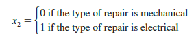
In regression analysis x2 is called a dummy or indicator variable. Using this dummy variable, we can write the multiple regression model as
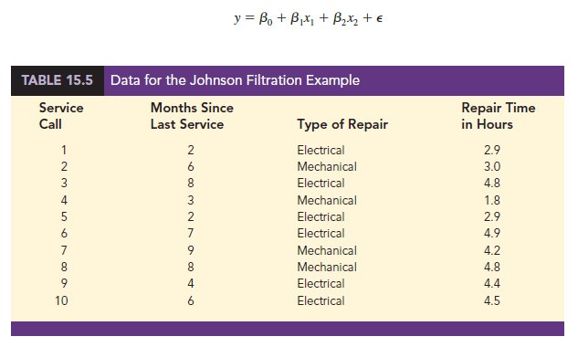
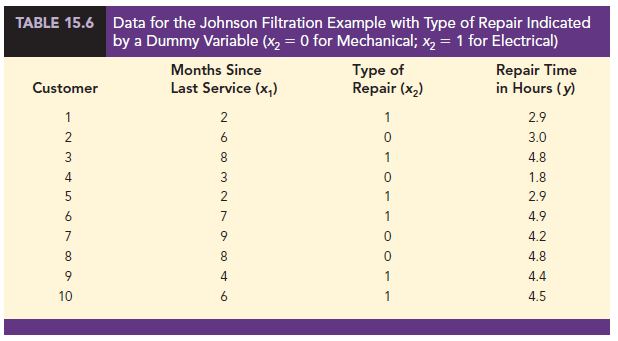
Table 15.6 is the revised data set that includes the values of the dummy variable. The output in Figure 15.8 shows that the estimated multiple regression equation is
![]()
At the .05 level of significance, the p-value of .001 associated with the F test (F = 21.36) indicates that the regression relationship is significant. The t test part of the output in
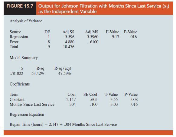
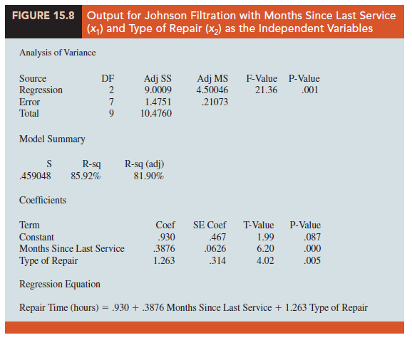
Figure 15.8 shows that both months since last service (p-value = .000) and type of repair (p-value = .005) are statistically significant. In addition, R-Sq = 85.92% and R-Sq (adj) = 81.9% indicate that the estimated regression equation does a good job of explaining the variability in repair times. Thus, equation (15.17) should prove helpful in predicting the repair time necessary for the various service calls.
2. Interpreting the Parameters
The multiple regression equation for the Johnson Filtration example is
![]()
To understand how to interpret the parameters b0, b1, and b2 when a categorical variable is present, consider the case when x2 = 0 (mechanical repair). Using E(y | mechanical) to denote the mean or expected value of repair time given a mechanical repair, we have
![]()
Similarly, for an electrical repair (x2 = 1), we have
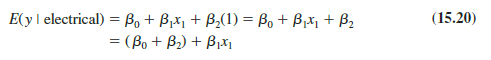
Comparing equations (15.19) and (15.20), we see that the mean repair time is a linear function of x1 for both mechanical and electrical repairs. The slope of both equations is $1, but the y-intercept differs. The y-intercept is β0 in equation (15.19) for mechanical repairs and (β0 + β2) in equation (15.20) for electrical repairs. The interpretation of β2 is that it indicates the difference between the mean repair time for an electrical repair and the mean repair time for a mechanical repair.
If β2 is positive, the mean repair time for an electrical repair will be greater than that for a mechanical repair; if β2 is negative, the mean repair time for an electrical repair will be less than that for a mechanical repair. Finally, if β2 = 0, there is no difference in the mean repair time between electrical and mechanical repairs and the type of repair is not related to the repair time.
Using the estimated multiple regression equation y = .93 + .3876x1 + 1.263x2, we see that .93 is the estimate of β0 and 1.263 is the estimate of β2. Thus, when x2 = 0 (mechanical repair)
![]()
and when x2 = 1 (electrical repair)
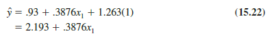
In effect, the use of a dummy variable for type of repair provides two estimated regression equations that can be used to predict the repair time, one corresponding to mechanical repairs and one corresponding to electrical repairs. In addition, with b2 = 1.263, we learn that, on average, electrical repairs require 1.263 hours longer than mechanical repairs.
Figure 15.9 is the plot of the Johnson data from Table 15.6. Repair time in hours (y) is represented by the vertical axis and months since last service (x1) is represented by the horizontal axis. A data point for a mechanical repair is indicated by an M and a data point for an electrical repair is indicated by an E. Equations (15.21) and (15.22) are plotted on the graph to show graphically the two equations that can be used to predict the repair time, one corresponding to mechanical repairs and one corresponding to electrical repairs.

3. More Complex Categorical Variables
Because the categorical variable for the Johnson Filtration example had two levels (mechanical and electrical), defining a dummy variable with zero indicating a mechanical repair and one indicating an electrical repair was easy. However, when a categorical variable has more than two levels, care must be taken in both defining and interpreting the dummy variables. As we will show, if a categorical variable has k levels, k — 1 dummy variables are required, with each dummy variable being coded as 0 or 1.
For example, suppose a manufacturer of copy machines organized the sales territories for a particular state into three regions: A, B, and C. The managers want to use regression analysis to help predict the number of copiers sold per week. With the number of units sold as the dependent variable, they are considering several independent variables (the number of sales personnel, advertising expenditures, and so on). Suppose the managers believe sales region is also an important factor in predicting the number of copiers sold. Because sales region is a categorical variable with three levels, A, B and C, we will need 3 — 1 = 2 dummy variables to represent the sales region. Each variable can be coded 0 or 1 as follows.
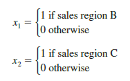
With this definition, we have the following values of x and x2.

Observations corresponding to region A would be coded Xj = 0, x2 = 0; observations corresponding to region B would be coded x1 = 1, x2 = 0; and observations corresponding to region C would be coded x1 = 0, x 2 = 1.
The regression equation relating the expected value of the number of units sold, E( y), to the dummy variables would be written as
![]()
To help us interpret the parameters β0, β1, and β2, consider the following three variations of the regression equation.

Thus, β0 is the mean or expected value of sales for region A; β1 is the difference between the mean number of units sold in region B and the mean number of units sold in region A; and β2 is the difference between the mean number of units sold in region C and the mean number of units sold in region A.
Two dummy variables were required because sales region is a categorical variable with three levels. But the assignment of x1 = 0, x2 = 0 to indicate region A, x1 = 1, x2 = 0 to indicate region B, and x1 = 0, x2 = 1 to indicate region C was arbitrary. For example, we could have chosen x1 = 1, x2 = 0 to indicate region A, x1 = 0, x2 = 0 to indicate region B, and x1 = 0, x2 = 1 to indicate region C. In that case, β1 would have been interpreted as the mean difference between regions A and B and β2 as the mean difference between regions C and B.
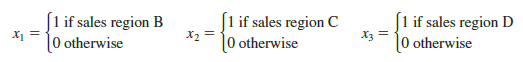
The important point to remember is that when a categorical variable has k levels, k – 1 dummy variables are required in the multiple regression analysis. Thus, if the sales region example had a fourth region, labeled D, three dummy variables would be necessary. For example, the three dummy variables can be coded as follows.
Source: Anderson David R., Sweeney Dennis J., Williams Thomas A. (2019), Statistics for Business & Economics, Cengage Learning; 14th edition.
30 Aug 2021
31 Aug 2021
30 Aug 2021
31 Aug 2021
31 Aug 2021
30 Aug 2021