Autocorrelation and the Durbin-Watson Test

Often, the data used for regression studies in business and economics are collected over time.

It is not uncommon for the value of y at time t, denoted by y, to be related to the value of y at previous time periods. In such cases, we say autocorrelation (also called serial correlation) is present in the data. If the value of y in time period t is related to its value in time period t – 1, first-order autocorrelation is present. If the value of y in time period t is related to the value of y in time period t – 2, second-order autocorrelation is present, and so on.

One of the assumptions of the regression model is the error terms are independent. How­ever, when autocorrelation is present, this assumption is violated. In the case of first-order autocorrelation, the error at time t, denoted ∈_t, will be related to the error at time period t – 1, denoted ∈_t-1. Two cases of first-order autocorrelation are illustrated in Figure 16.19. Panel A is the case of positive autocorrelation; panel B is the case of negative autocor­relation. With positive autocorrelation we expect a positive residual in one period to be followed by a positive residual in the next period, a negative residual in one period to be followed by a negative residual in the next period, and so on. With negative autocorrelation, we expect a positive residual in one period to be followed by a negative residual in the next period, then a positive residual, and so on.

When autocorrelation is present, serious errors can be made in performing tests of statistical significance based upon the assumed regression model. It is therefore import­ant to be able to detect autocorrelation and take corrective action. We will show how the Durbin-Watson statistic can be used to detect first-order autocorrelation.

Suppose the values of e are not independent but are related in the following manner:

where p is a parameter with an absolute value less than one and z_t is a normally and inde­pendently distributed random variable with a mean of zero and a variance of σ². From equa­tion (16.16) we see that if p = 0, the error terms are not related, and each has a mean of zero and a variance of σ². In this case, there is no autocorrelation and the regression assumptions are satisfied. If p > 0, we have positive autocorrelation; if p < 0, we have negative autocor­relation. In either of these cases, the regression assumptions about the error term are violated.

The Durbin-Watson test for autocorrelation uses the residuals to determine whether p = 0. To simplify the notation for the Durbin-Watson statistic, we denote the ith residual by e, = yi – y_t. The Durbin-Watson test statistic is computed as follows:

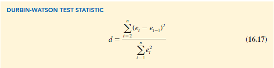
If successive values of the residuals are close together (positive autocorrelation), the value of the Durbin-Watson test statistic will be small. If successive values of the residuals are far apart (negative autocorrelation), the value of the Durbin-Watson statistic will be large.

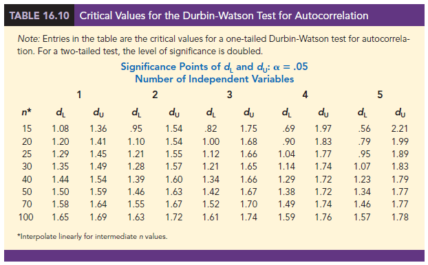
The Durbin-Watson test statistic ranges in value from zero to four, with a value of two indicating no autocorrelation is present. Durbin and Watson developed tables that can be used to determine when their test statistic indicates the presence of autocorrelation. Table 16.10 shows lower and upper bounds (d_L and d_∪) for hypothesis tests using a = .05; n denotes the number of observations. The null hypothesis to be tested is always that there is no autocorrelation.

The alternative hypothesis to test for positive autocorrelation is

The alternative hypothesis to test for negative autocorrelation is

A two-sided test is also possible. In this case the alternative hypothesis is

Figure 16.20 shows how the values of d_L and d_∪ in Table 16.10 are used to test for auto­correlation. Panel A illustrates the test for positive autocorrelation. If d < d_L, we conclude that positive autocorrelation is present. If d_L ≤ d ≤ d_∪, we say the test is inconclusive. If d > d_∪, we conclude that there is no evidence of positive autocorrelation.

Panel B illustrates the test for negative autocorrelation. If d > 4 – d_L, we conclude that negative autocorrelation is present. If 4 – d_∪ ≤ d ≤ 4 – d_L, we say the test is inconclusive. If d < 4 – d_∪, we conclude that there is no evidence of negative autocorrelation.

Panel C illustrates the two-sided test. If d < d_L or d > 4 – d_L, we reject H₀ and con­clude that autocorrelation is present. If d_L ≤ d ≤ d_∪ or 4 – d_∪ < d < 4 – d_L, we say the test is inconclusive. If d_∪ < d < 4 – d_∪, we conclude that there is no evidence of autocorrelation.

If significant autocorrelation is identified, we should investigate whether we omitted one or more key independent variables that have time-ordered effects on the dependent variable. If no such variables can be identified, including an independent variable that measures the time of the observation (for instance, the value of this variable could be one for the first observation, two for the second observation, and so on) will sometimes eliminate or reduce the autocorrelation. When these attempts to reduce or remove auto­correlation do not work, transformations on the dependent or independent variables can prove helpful; a discussion of such transformations can be found in more advanced texts on regression analysis.

Note that the Durbin-Watson tables list the smallest sample size as 15. The reason is that the test is generally inconclusive for smaller sample sizes; in fact, many statist­icians believe the sample size should be at least 50 for the test to produce worthwhile results.

Source:  Anderson David R., Sweeney Dennis J., Williams Thomas A. (2019), Statistics for Business & Economics, Cengage Learning; 14th edition.