Pricing and Revenue Management for Perishable Assets in a Supply Chain

Any asset that loses value over time is perishable. Clearly, fruits, vegetables, and pharmaceuti­cals are perishable, but this list also includes products such as computers and cell phones that lose value as new models are introduced. High-fashion apparel is perishable because it cannot be sold at full price once the season is past. Perishable assets also include all forms of production, transportation, and storage capacity that is wasted if not fully utilized. Unused capacity from the past has no value. Thus, all unused capacity is equivalent to perished capacity.

A well-known example of revenue management in retailing of apparel was the original Filene’s Basement in Boston. Merchandise was first sold at the main store at full price. Leftover merchandise was moved to the basement and its price reduced incrementally over a 35-day period until it sold. Any unsold merchandise was then given away to charity. Today, most depart­ment stores progressively discount merchandise over the sales season and then sell any remain­ing inventory to an outlet store, which follows a similar pricing strategy.

Another example of revenue management for a perishable asset is the use of overbooking by the airline industry. An airplane seat loses all value once the plane takes off. Given that people often do not show up for a flight even when they have a reservation, airlines sell more reserva­tions than the capacity of the plane, to maximize expected revenue.

The following are two revenue management tactics used for perishable assets:

1. Vary price dynamically over time to maximize expected revenue.
2. Overbook sales of the asset to account for cancellations.

1. Dynamic Pricing

Dynamic pricing, the tactic of varying price over time, is suitable for assets such as fashion apparel that have a clear date beyond which they lose much of their value. The success of dynamic pricing also requires the presence of different customer segments, with some willing to pay a higher price for the product. Apparel designed for the winter does not have much value by April. A retailer that has purchased 100 ski jackets in October has many options with regard to its pricing strategy. It can charge a high price initially. This strategy will attract only customers with a high willingness to pay and will result in fewer sales early in the season (though at a higher price), leaving more jackets to be sold later during the season. A discount later in the season can then attract customers who have a lower value for the product. Another option is to charge a lower price initially, selling more jackets early in the season (though at a lower price) and leaving fewer jackets to be sold at a discount. This trade-off determines the profits for the retailer. To vary price effectively over time for a perishable asset, the asset owner must be able to estimate the value of the asset over time and forecast the impact of price on customer demand effectively. Effective differential pricing over time generally increases the level of product availability for the consumer willing to pay full price and also increases total profits for the retailer.

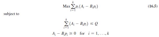
We now discuss a simple methodology for dynamic pricing when the seller has a speci­fied quantity Q of a single product at the start of the season. We assume that the seller is able to divide the selling season into k periods and can forecast the demand curve for each period. The underlying assumptions here are that customers’ responses to pricing can be predicted over time and customers will not change their behavior in response to anticipated price changes. For simplicity, we assume that given a price p_; in period i, the demand d_i in period i is given by

di = Ai – Bipi

This is a linear demand curve, but in general the demand curve need not be linear. We pres­ent the linear case here because it is easier to understand and solve. The assumption is that cus­tomers that purchase in the initial periods are less price sensitive, whereas those that purchase later are more price sensitive. The retailer wants to vary the price over time to maximize the revenue it can extract from the Q units it has on hand at the beginning of the season. The dynamic pricing problem faced by the retailer can then be formulated as follows:

As formulated, the dynamic pricing problem is simple enough that it can be solved directly using Excel as illustrated in Example 16-3 [see worksheets Example16-3(dynamic price) and Example16-3(fixed price)].

EXAMPLE 16-3 Dynamic Pricing

A retailer has purchased 400 ski parkas before the start of the winter season at a cost of $100 each (for a total cost of $40,000). The season lasts three months, and the retailer has forecast demand in each of the three months to be di = 300 – p₁, d₂ = 300 – 1.3p₂, and d₃ = 300 – 1.8p₃. How should the retailer vary the price of the parka over the three months to maximize revenue? If the retailer charges a constant price over the three months, what should it be? How much gain in profit results from dynamic pricing?

Analysis:

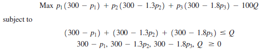
Observe that customers who buy at the beginning of the season are forecast to be less price sensi­tive and customers who buy toward the end of the season are more price sensitive. Using Equa­tion 16.5, the retailer’s problem can be formulated as follows:

Maxp₁(300 – p₁) + p₂(300 – 1.3p₂) + p₃(300 – 1.8p₃)

subject to

This problem can be formulated using Solver in Excel, as shown in Figure 16-4 [see worksheet Example16-3(dynamic price)]. Cells B5:B7 contain the price variables, cells C5:C7 contain the resulting demand from the respective demand curves, and cells D5:D7 contain the revenue in each period. The total demand across the three periods is in cell C8 and the total revenue is in cell D8. The quantity at the beginning of the season is in cell B3.

As shown in Figure 16-4, the optimal strategy for the retailer is to price at $162.20 in the first month, $127.58 in the second month, and $95.53 in the third month. This gives total revenue of $51,697.94 and profit of $11,697.94 for the retailer.

The problem of obtaining the optimal fixed price over the three-month season can be for­mulated in Excel as shown in Figure 16-5 [see worksheet Example16-3(fixed price)]. All cell formulas except B6 and B7 are as in Figure 16-4.

If the retailer wants to have a fixed price over the three months, it should price the jackets at $121.95 for resulting revenue of $48,780.49 and profit of $8,780.49. We can see that dynamic pricing allows the retailer to increase profits by almost $3,000, from $8,780 to $11,698.

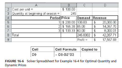
Once we have understood how to price the product dynamically over the season, we can go back and ask how many units the retailer should purchase at the beginning of the season to maximize profits, as described in Example 16-4 (see worksheet Example16-4).

EXAMPLE 16-4 Evaluating Quantity with Dynamic Pricing

Return to the retailer in Example 16-3. Assume demand curves as described in Example 16-3. How many parkas should the retailer purchase at the beginning of the season, and how should they be priced over the three months of the season to maximize profits?

Analysis:

In this case, the quantity at the beginning of the season is also a decision variable. The retailer’s problem can now be formulated as follows:

The problem can be formulated in Excel as shown in Figure 16-6 (see worksheet Example16-4) to obtain the optimal initial quantity and dynamic prices over the season. All cell formulas except cell D9 are as in Figure 16-4.

It is optimal for the retailer to order 245 jackets at the beginning of the season. They are then priced at $200 for the first month, $165.38 for the second month, and $133.33 for the third month. The total profit for the retailer with the optimal order quantity and dynamic pricing is $17,557.69. Observe that this is higher than the profit obtained in Example 16-4 when the retailer started the season with 400 parkas.

Although dynamic pricing can seem very profitable as long as customers do not anticipate price decreases and delay their purchases, the situation is more challenging when customers choose to behave strategically and delay their purchases to wait for a lower price.

THE CHALLENGE OF STRATEGIC CUSTOMERS In reality, the dynamic pricing problem is more complicated because demand is unpredictable and customers behave strategically in that they may decide to delay their purchases if they know that prices will drop over time. An excellent discussion of models that can be used in this more complex setting can be found in Talluri and Van Ryzin (2004).

The issue of unpredictable demand and strategic customers is illustrated effectively in decisions made by the high-end retailer Saks Fifth Avenue in November 2008. In 2007, luxury goods from brands such as Prada, Gucci, and Dolce & Gabbana had become especially impor­tant for high-end retailers such as Saks, which maintained strong sales into mid-2008 even though retailing overall was starting to drop by then. As a result, Saks placed its orders for the holiday season of 2008 hoping for strong sales of these brands. By November, however, a huge disconnect existed between inventories at Saks and customer demand. At Saks’s annual “private sale nights” in early November for top customers, the usual 40 percent discounts got no response. By mid-November, competitors such as Neiman Marcus had also dropped prices by 40 percent and some designers were offering 90 percent discounts in “sample sales.” The more prices dropped, the more customers decided to delay their purchases in anticipation of even lower prices. As Thanksgiving approached, Saks decided to offer 70 percent discounts to move its inventory.

When there is a lot of inventory at a retailer, it is reasonable to expect that some customers will be strategic and delay their purchase in anticipation of a lower price in the future. Ignoring this strategic behavior by customers can significantly reduce the benefits of dynamic pricing for retailers. Consider, for example, the retailer in Example 16-4 that starts the season with 245 units, as suggested by the results of Example 16-4. When customers are not strategic, the retailer expects to sell 100 units at $200 each in the first month, 85 units at $165.38 each in the second month, and the remaining 60 units at $133.33 each in the third month, for total sales of $42,057.71 and a profit of $17,557.08 (given a unit cost of $100). Now consider the case of strategic customers detailed in the worksheet Example16-4(strategic). If strategic customers delay their purchase and the retailer sells only 80 units in the first month and 50 in the second month, the retailer is left with 115 units to be sold in the third month. To sell all 115 units, the retailer is forced to drop price in the third month to (300 – 115)/1.8 = $102.78. The total profit in this case drops to $11,588.43. The more that strategic customers wait until the third month, the bigger the drop in profits the retailer experi­ences. Clearly, the retailer pays a price for ignoring strategic customers.

In the presence of strategic customers, the retailer is better off buying 245 units and charg­ing a fixed price of $159.76 for the entire season [see worksheet Example16-4(fixedprice)]. The fixed price eliminates any gains for a customer from strategic behavior. At this price, the custom­ers buying in the first month purchase about 140 units, the customers buying in the second month purchase about 92 units, and only about 13 units are left to be sold in the third month. The retailer makes a total profit of $14,640 with a fixed price. Although this is lower than what the retailer would achieve with dynamic pricing if customers were not strategic, it is higher than potential profits with strategic customers. A credible fixed price can be an effective response to strategic customers. Tiffany is an example of a company that maintains this policy of a fixed price. Another approach is to reduce the quantity offered at the beginning of the season so cus­tomers are reluctant to take the risk of waiting for a late-season discount in case the entire quan­tity is sold out at full price. Zara uses this approach to get its customers to buy products when they see them on the shelf.

Key Point

Dynamic pricing can be a powerful tool to increase profits if the customers’ sensitivity to price changes in the course of the season. This is often the case for fashion products, for which customers are less price sensitive early in the season but become more price sensitive toward the end of the season. Dynamic pricing should, however, carefully consider strategic behavior by customers who may anticipate future price drops and delay their purchase. With strategic customers it may be better to have a fixed price or reduce the quantity offered.

2. Overbooking

Overbooking occurs when a seller with limited capacity sells more units than it has. Airlines often overbook to ensure that planes do not leave with empty seats. The tactic of overbooking or overselling of the available asset is suitable in any situation in which customers are able to cancel orders and the value of the asset drops significantly after a deadline. Examples include airline seats, items designed specially for Christmas, and production capacity. In each case, a limited amount of the asset is available, customers are allowed to cancel orders, and the asset loses value beyond a certain date. If the cancellation rate can be predicted accurately, the overbooking level is easy to determine. In practice, however, the cancellation rate is uncertain.

The basic trade-off to consider during overbooking is between having wasted capacity (or inventory) because of excessive cancellations or having a shortage of capacity (or inven­tory) because of few cancellations, in which case an expensive backup needs to be arranged. The cost of wasted capacity is the margin that would have been generated if the capacity had been used for production. The cost of a capacity shortage is the loss per unit that results from having to go to a backup source. The goal when making the overbooking decision is to maxi­mize supply chain profits by minimizing the cost of wasted capacity and the cost of capacity shortage.

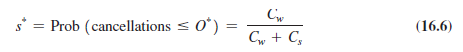
We now develop this trade-off in terms of a formula that can be used to set overbooking levels for an asset. Let p be the price at which each unit of the asset is sold, and let c be the cost of using or producing each unit of the asset. In case of asset shortage, let b be the cost per unit at which a backup can be used. Thus, the marginal cost of having wasted capacity is C_w = p — c, and the marginal cost of having a capacity shortage is C_s = b — p. If the cost of backup capacity is less than the sale price, there is no reason to limit the overbooking. The interesting case arises when the cost of backup capacity exceeds the sale price. The trade-off to obtain the optimal over­booking level is similar to the trade-off given by Equation 13.1 to obtain the optimal cycle ser­vice level for seasonal items. Let O* be the optimal overbooking level, and let / be the probability that cancellations will be less than or equal to O*. Similar to the derivation of Equa­tion 13.1, the optimal overbooking level is obtained as

If the distribution of cancellations is known in absolute terms to be normally distributed, with a mean of m_c and a standard deviation of s_c, the optimal overbooking level is evaluated as

If the cancellation distribution is known only as a function of the booking level (capacity L + overbooking O) to have a mean of m (L + O) and a standard deviation of s (L + O), the opti­mal overbooking level is obtained as a solution to the following equation:

Observe that the optimal level of overbooking should increase as the margin per unit increases, and the level of overbooking should decrease as the cost of replacement capacity goes up. Also observe that the use of overbooking increases asset utilization by customers. The use of overbooking decreases the number of customers that are turned away and thus improves asset availability to the customer, while improving profits for the asset owner. The evaluation of over­booking is illustrated in Example 16-5 (see worksheet Example16-5).

EXAMPLE 16-5 Overbooking

Consider an apparel supplier that is taking orders for dresses with a Christmas motif. The pro­duction capacity available from the supplier is 5,000 dresses, and it makes $10 for each dress sold. The supplier is currently taking orders from retailers and must decide on how many orders to commit to at this time. If it has orders that exceed capacity, it must arrange for backup capacity that results in a loss of $5 per dress.

Retailers have been known to cancel their orders near the winter season as they have better visibility into expected demand. How many orders should the supplier accept if cancellations are normally distributed, with a mean of 800 and a standard deviation of 400? How many orders should the supplier accept if cancellations are normally distributed, with a mean of 15 percent of the orders accepted and a coefficient of variation of 0.5?

Analysis:

The supplier has the following parameters:

Cost of wasted capacity, C_w = $10 per dress

Cost of capacity shortage, C_s = $5 per dress

Using Equation 16.6, we thus obtain

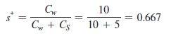
If cancellations are normally distributed, with a mean of 800 and a standard deviation of 400, the optimal overbooking level is obtained using Equation 16.7 as

In this case, the supplier should overbook by 972 dresses and take orders for a total of 5,972 dresses.

If cancellations are normally distributed with a mean of 15 percent of the booking level and a coefficient of variation of 0.5, the optimal overbooking level is obtained using Equation 16.8 to be the solution of the following equation:

This equation can be solved using Excel (see worksheet Example16-5) to obtain the optimal overbooking level:

O* = 1,115

In this case, the supplier should overbook by 1,115 dresses and take an order for up to 6,115 dresses.

Overbooking has been used as a tactic in the airline, passenger rail, and hotel industries. It has not, however, been used to the extent that it should be in many supply chain scenarios, including production, warehousing, and transportation capacity. There is no reason that a third- party warehouse that rents to multiple customers should not sell total space that exceeds the available space. A backup will clearly be needed if all customers use warehouse space to capac­ity. In all other cases, the available warehouse capacity will cover the need for space. Overbook­ing in this case will improve revenues for the warehouse while allowing more customers to use the available warehouse space.

Source: Chopra Sunil, Meindl Peter (2014), Supply Chain Management: Strategy, Planning, and Operation, Pearson; 6th edition.