In any global supply chain, demand, prices, exchange rates, and several other factors are uncertain and are likely to fluctuate during the life of any supply chain decision. In an uncertain environment, the problem with using a simple DCF analysis is that it typically undervalues flexibility. The result is often a supply chain that performs well if everything goes according to plan but becomes terribly expensive if something unexpected happens. A manager makes several different decisions when designing a supply chain network. For instance:
- Should the firm sign a long-term contract for warehousing space or get space from the spot market as needed?
- What should the firm’s mix of long-term and spot market be in the portfolio of transportation capacity?
- How much capacity should various facilities have? What fraction of this capacity should be flexible?
If uncertainty is ignored, a manager will always sign long-term contracts (because they are typically cheaper) and avoid all flexible or backup capacity (because it is more expensive). Such decisions can hurt the firm, however, if future demand or prices are not as forecast at the time of the decision. Executives participating in the Accenture 2013 Global Manufacturing Study “cited a variety of volatility-related factors as potential impediments to their ability to grow—including global currency instability, unpredictable commodities costs, uncertainty about customer demand, political or social unrest in key markets, and potential changes in government regulations.” It is thus important to provide a methodology that allows managers to incorporate this uncertainty into their network design process. In this section, we describe such a methodology and show that accounting for uncertainty can have a significant impact on the value of network design decisions.
1. The Basics of Decision Tree Analysis
A decision tree is a graphic device used to evaluate decisions under uncertainty. Decision trees with DCFs can be used to evaluate supply chain design decisions given uncertainty in prices, demand, exchange rates, and inflation.
The first step in setting up a decision tree is to identify the number of time periods into the future that will be considered when making the decision. The decision maker should also identify the duration of a period—a day, a month, a quarter, or any other time period. The duration of a period should be the minimum period of time over which factors affecting supply chain decisions may change by a significant amount. “Significant” is hard to define, but in most cases it is appropriate to use as a period the duration over which an aggregate plan holds. If planning is done monthly, for example, we set the duration of a period at a month. In the following discussion, T will represent the number of time periods over which the supply chain decision is to be evaluated.
The next step is to identify factors that will affect the value of the decision and are likely to fluctuate over the next T periods. These factors include demand, price, exchange rate, and inflation, among others. Having identified the key factors, the next step is to identify probability distributions that define the fluctuation of each factor from one period to the next. If, for instance, demand and price are identified as the two key factors that affect the decision, the probability of moving from a given value of demand and price in one period to any other value of demand and price in the next period must be defined.
The next step is to identify a periodic discount rate k to be applied to future cash flows. It is not essential that the same discount rate apply to each period or even at every node in a period. The discount rate should take into account the inherent risk associated with the investment. In general, a higher discount rate should apply to investments with higher risk.
The decision is now evaluated using a decision tree, which contains the present and T future periods. Within each period, a node must be defined for every possible combination of factor values (say, demand and price) that can be achieved. Arrows are drawn from origin nodes in Period i to end nodes in Period i + 1. The probability on an arrow is referred to as the transition probability and is the probability of transitioning from the origin node in Period i to the end node in Period i + 1.
The decision tree is evaluated starting from nodes in Period T and working back to Period
- For each node, the decision is optimized, taking into account current and future values of various factors. The analysis is based on Bellman’s principle, which states that for any choice of strategy in a given state, the optimal strategy in the next period is the one that is selected if the entire analysis is assumed to begin in the next period. This principle allows the optimal strategy to be solved in a backward fashion starting at the last period. Expected future cash flows are discounted back and included in the decision currently under consideration. The value of the node in Period 0 gives the value of the investment, as well as the decisions made during each time period. (Tools such as Treeplan are available that help solve decision trees on spreadsheets.) The decision tree analysis methodology is summarized as follows:
- Identify the duration of each period (month, quarter, etc.) and the number of periods T over which the decision is to be evaluated.
- Identify factors such as demand, price, and exchange rate whose fluctuation will be considered over the next T
- Identify representations of uncertainty for each factor; that is, determine what distribution to use to model the uncertainty.
- Identify the periodic discount rate k for each period.
- Represent the decision tree with defined states in each period, as well as the transition probabilities between states in successive periods.
- Starting at period T, work back to Period 0, identifying the optimal decision and the expected cash flows at each step. Expected cash flows at each state in a given period should be discounted back when included in the previous period.
2. Evaluating Flexibility at Trips Logistics
We illustrate the decision tree analysis methodology by using the lease decision facing the general manager at Trips Logistics. The manager must decide whether to lease warehouse space for the coming three years and the quantity to lease. The manager anticipates uncertainty in demand and spot prices for warehouse space over the coming three years. The long-term lease is cheaper but the space could go unused if demand is lower than anticipated. The long-term lease may also end up being more expensive if future spot market prices come down. The manager is considering three options:
- Get all warehousing space from the spot market as needed.
- Sign a three-year lease for a fixed amount of warehouse space and get additional requirements from the spot market.
- Sign a flexible lease with a minimum charge that allows variable usage of warehouse space up to a limit, with additional requirements from the spot market.
We now discuss how the manager can evaluate each decision, taking uncertainty into account. One thousand square feet of warehouse space is required for every 1,000 units of demand, and the current demand at Trips Logistics is for 100,000 units per year. The manager forecasts that from one year to the next, demand may go up by 20 percent, with a probability of 0.5, or go down by 20 percent, with a probability of 0.5. The probabilities of the two outcomes are independent and unchanged from one year to the next.
The general manager can sign a three-year lease at a price of $1 per square foot per year. Warehouse space is currently available on the spot market for $1.20 per square foot per year.

From one year to the next, spot prices for warehouse space may go up by 10 percent, with probability 0.5, or go down by 10 percent, with probability 0.5. The probabilities of the two outcomes are independent and unchanged from one year to the next.
The general manager believes that prices of warehouse space and demand for the product fluctuate independently. Each unit Trips Logistics handles results in revenue of $1.22, and Trips Logistics is committed to handling all demand that arises. Trips Logistics uses a discount rate of k = 0.1 for each of the three years.
The general manager assumes that all costs are incurred at the beginning of each year and thus constructs a decision tree with T = 2. The decision tree is shown in Figure 6-2, with each node representing demand (D) in thousands of units and price (p) in dollars. The probability of each transition is 0.5 X 0.5 = 0.25 because price and demand fluctuate independently.
3. Evaluating the Spot Market Option
Using the decision tree in Figure 6-2, the manager first analyzes the option of not signing a lease and obtaining all warehouse space from the spot market. He starts with Period 2 and evaluates the profit for Trips Logistics at each node. At the node D = 144, p = $1.45, Trips Logistics must satisfy a demand of 144,000 and faces a spot price of $1.45 per square foot for warehouse space in Period 2. The cost incurred by Trips Logistics in Period 2 at the node D = 144, p = $1.45 is represented by C(D = 144, p =1.45, 2) and is given by

C(D = 144, p = 1.45, 2) = 144,000 X 1.45 = $208,800
The profit at Trips Logistics in Period 2 at the node D = 144, p = $1.45 is represented by P(D = 144, p = 1.45, 2) and is given by
P(D = 144,p = 1.45, 2) = 144,000 X 1.22 – C(D = 144,p = 1.45, 2)
= 175,680 – 208,800 = -$33,120
The profit for Trips Logistics at each of the other nodes in Period 2 is evaluated similarly, as shown in Table 6-5.
The manager next evaluates the expected profit at each node in Period 1 to be the profit during Period 1 plus the present value (in Period 1) of the expected profit in Period 2. The expected profit EP(D =, p =, 1) at a node is the expected profit over all four nodes in Period 2 that may result from this node. PVEP(D =, p =, 1) represents the present value of this expected profit; P(D =, p =, 1), the total expected profit, is the sum of the profit in Period 1 and the present value of the expected profit in Period 2. From the node D = 120, p = $1.32 in Period 1, there are four possible states in Period 2. The manager thus evaluates the expected profit in Period 2 over all four states possible from the node D = 120, p = $1.32 in Period 1 to be EP(D = 120, p = 1.32, 1),
where
EP(D = 120, p = 1.32, 1) = 0.25 X [P(D = 144, p = 1.45, 2) + P(D = 144, p = 1.19, 2) + P(D = 96, p = 1.45, 2) + P(D = 96, p = 1.19, 2) ]
= 0.25 X [-33,120 + 4,320 – 22,080 + 2,880]
= -$12,000
The present value of this expected value in Period 1 is given by
PVEP(D = 120, p = 1.32, 1) = EP(D = 120, p = 1.32, 1)/(1 + k)
= -12,000 / 1.1 = – $10,909
The manager obtains the total expected profit P(D = 120, p = 1.32, 1) at node D = 120, p = 1.32 in Period 1 to be the sum of the profit in Period 1 at this node and the present value of future expected profits.

P(D = 120, p = 1.32, 1) = (120,000 X 1.22) – (120,000 X 1.32) + PVEP(D = 120, p = 1.32, 1) = – $12,000 – $10,909 = – $22,909
The total expected profit for all other nodes in Period 1 is evaluated as shown in Table 6-6.
For Period 0, the total profit P(D = 100, p = 1.20, 0) is the sum of the profit at Period 0 and the present value of the expected profit over the four nodes in Period 1.
EP(D = 100,p = 1.20, 0) = 0.25 X [P(D = 120,p = 1.32, 1) + P(D = 120,p = 1.08, 1) + P(D = 80, p = 1.32, 1) + P(D = 80, p = 1.08, 1)] = 0.25 X [ -22,909 + 32,073 – 15,273 + 21,382]
= $3,818 PVEP(D = 100, p = 1.20, 0) = EP(D = 100, p = 1.20, 0)/( 1 + k)
= 3,818 / 1.1 = $3,471
P(D = 100,p = 1.20, 0) = (100,000 X 1.22) – (100,000 X 1.20) + PVEP(D = 100, p = 1.20, 0) = $2,000 + $3,471 = $5,471
Thus, the expected NPV of not signing the lease and obtaining all warehousing space from the spot market is
NPV (Spot Market) = $5,471
4. Evaluating the Fixed Lease Option
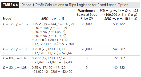
The manager next evaluates the alternative whereby the lease for 100,000 sq. ft. of warehouse space is signed. The evaluation procedure is very similar to that for the previous case, but the outcome changes in terms of profit. For example, at the node D = 144, p = 1.45, the manager will require 44,000 square feet of warehouse space from the spot market at $1.45 per square foot because only 100,000 square feet have been leased at $1 per square foot. If demand happens to be less than 100,000 units, Trips Logistics still has to pay for the entire 100,000 square feet of leased space. For Period 2, the manager obtains the profit at each of the nine nodes, as shown in Table 6-7.
The manager next evaluates the total expected profit for each node in Period 1. Again, the expected profit EP(D =, p =, 1) at a node is the expected profit of all four nodes in Period 2 that may result from this node (see Figure 6-2), and P(D =, p =, 1) is the total expected profit from both Periods 1 and 2. The manager thus obtains the results in Table 6-8.
For Period 0, the expected profit EP(D = 100, p = 1.20, 0) over the four nodes in Period 1 is given by
EP(D = 100,p = 1.20, 0) = 0.25 X [P(D = 120,p = 1.32, 1) + P(D = 120,p = 1.08, 1) + P(D = 80, p = 1.32, 1) + P(D = 80, p = 1.08, 1)]
= 0.25 X [35,782 + 45,382 – 4,582 – 4,582] = $18,000

The present value of the expected profit in Period 0 is given by
PVEP(D = 100, p = 1.20, 0) = EP(D = 100, p = 1.20, 0)/(1 + k)
= 18,000/ 1.1 = $16,364
The total expected profit is obtained as the sum of the profit in Period 0 and the present value of the expected profit over all four nodes in Period 1. It is
P(D = 100,p = 1.20, 0) = (100,000 X 1.22) – (100,000 X 1) + PVEP(D = 100, p = 1.20, 0) = $22,000 + $16,364 = $38,364
The NPV of signing a three-year lease for 100,000 sq. ft. of warehouse space is thus
NPV( Lease) = $38,364
Observe that the NPV of the lease option under uncertainty is considerably less compared to when uncertainty is ignored ($60,182 from Example 6-1). This is because the lease is a fixed decision, and Trips Logistics is unable to react to market conditions by leasing less space if demand is lower. Rigid contracts are less attractive in the presence of uncertainty.
5. Evaluating the Flexible Lease Option
The general manager at Trips Logistics has been offered a contract in which, for an upfront payment of $10,000, Trips Logistics will have the flexibility of using between 60,000 square feet and 100,000 square feet of warehouse space at $1 per square foot per year. Trips Logistics must pay $60,000 per year for the first 60,000 square feet and can then use up to another 40,000 square feet on demand at $1 per square foot. The general manager decides to use decision trees to evaluate whether this flexible contract is preferable to a fixed contract for 100,000 square feet.
The underlying decision tree for evaluating the flexible contract is exactly as in Figure 6-2. The profit at each node, however, changes because of the flexibility in space used as shown in Table 6-9. If demand is larger than 100,000 units, Trips Logistics uses all 100,000 square feet of warehouse space at $1 and gets the rest at the spot price. If demand is between 60,000 and 100,000 units, Trips Logistics uses and pays $1 only for the exact amount of warehouse space required. The profit at all nodes where demand is 100,000 or higher remains the same as in Table 6-7. The profit in Period 2 at all nodes where demand is less than 100,000 units increases as shown in Table 6-9.
The general manager evaluates the expected profit EP(D =, p =, 1) from Period 2 and the total expected profit for each node in Period 1, as discussed earlier. The results are shown in Table 6-10.
The total expected profit in Period 0 is the sum of the profit in Period 0 and the present value of the expected profit in Period 1. The manager thus obtains
EP(D = 100,p = 1.20, 0) = 0.25 X [P(D = 120,p = 1.32, 1) + P(D = 120,p = 1.08, 1) + P(D = 80, p = 1.32, 1) + P(D = 80, p = 1.08, 1)]
= 0.25 X [37,600 + 47,200 + 33,600 + 33,600]
= $38,000 PVEP( D = 100, p = 1.20, 1)
= EP(D = 100, p = 1.20, 0)/(1 + k)
= 38,000/ 1.1 = $34,545
P(D = 100,p = 1.20, 0) = (100,000 X 1.22) – (100,000 X 1) + PVEP(D = 100, p = 1.20, 0) = $22,000 + $34,545 = $56,545

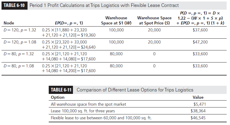
With an upfront payment of $10,000, the net expected profit is $46,545 under the flexible lease. Accounting for uncertainty, the manager at Trips Logistics values the three options as shown in Table 6-11.
The flexible contract is thus beneficial for Trips Logistics because it is $8,181 more valuable than the rigid contract for three years.
Source: Chopra Sunil, Meindl Peter (2014), Supply Chain Management: Strategy, Planning, and Operation, Pearson; 6th edition.
Aweѕome poѕt.
Sweet website , super design and style, really clean and apply genial.