We saw earlier (see Figure 7.1— page 239) that short-run average cost curves are U-shaped. We will see that long-run average cost curves can also be U-shaped, but different economic factors explain the shapes of these curves. In this section, we discuss long-run average and marginal cost curves and highlight the differ- ences between these curves and their short-run counterparts.
1. The Inflexibility of Short-Run Production
Recall that we defined the long run as occurring when all inputs to the firm are variable. In the long run, the firm’s planning horizon is long enough to allow for a change in plant size. This added flexibility allows the firm to produce at a lower average cost than in the short run. To see why, we might compare the situation in which capital and labor are both flexible to the case in which capi- tal is fixed in the short run.
Figure 7.8 shows the firm’s production isoquants. The firm’s long-run expan- sion path is the straight line from the origin that corresponds to the expansion path in Figure 7.6. Now, suppose capital is fixed at a level K1 in the short run. To produce output q1, the firm would minimize costs by choosing labor equal to L1, corresponding to the point of tangency with the isocost line AB. The inflexibility appears when the firm decides to increase its output to q2 without increasing its use of capital. If capital were not fixed, it would produce this output with capital K2 and labor L2. Its cost of production would be reflected by isocost line CD.
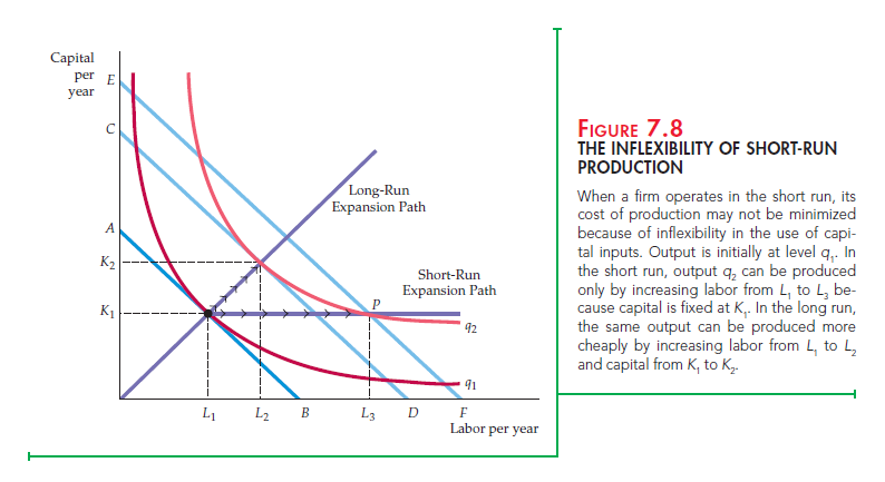
However, the fact that capital is fixed forces the firm to increase its output by using capital K1 and labor L3 at point P. Point P lies on the isocost line EF, which represents a higher cost than isocost line CD. Why is the cost of production higher when capital is fixed? Because the firm is unable to substitute relatively inexpensive capital for more costly labor when it expands production. This inflexibility is reflected in the short-run expansion path, which begins as a line from the origin and then becomes a horizontal line when the capital input reaches K1.
2. Long–Run Average Cost
In the long run, the ability to change the amount of capital allows the firm to reduce costs. To see how costs vary as the firm moves along its expansion path in the long run, we can look at the long-run average and marginal cost curves.9 The most important determinant of the shape of the long-run average and marginal cost curves is the relationship between the scale of the firm’s operation and the inputs that are required to minimize its costs. Suppose, for example, that the firm’s production process exhibits constant returns to scale at all input levels. In this case, a doubling of inputs leads to a doubling of output. Because input prices remain unchanged as output increases, the average cost of production must be the same for all levels of output.
Suppose instead that the firm’s production process is subject to increasing returns to scale: A doubling of inputs leads to more than a doubling of output. In that case, the average cost of production falls with output because a doubling of costs is associated with a more than twofold increase in output. By the same logic, when there are decreasing returns to scale, the average cost of production must be increasing with output.
We saw that the long-run total cost curve associated with the expansion path in Figure 7.6 (a) was a straight line from the origin. In this constant-returns-to-scale case, the long-run average cost of production is constant: It is unchanged as out- put increases. For an output of 100, long-run average cost is $1000/100 = $10 per unit. For an output of 200, long-run average cost is $2000/200 = $10 per unit; for an output of 300, average cost is also $10 per unit. Because a constant average cost means a constant marginal cost, the long-run average and marginal cost curves are given by a horizontal line at a $10/unit cost.
Recall that in the last chapter we examined a firm’s production technology that exhibits first increasing returns to scale, then constant returns to scale, and eventually decreasing returns to scale. Figure 7.9 shows a typical long-run aver- age cost curve (LAC) consistent with this description of the production process. Like the short-run average cost curve (SAC), the long-run average cost curve is U-shaped, but the source of the U-shape is increasing and decreasing returns to scale, rather than diminishing returns to a factor of production.
The long-run marginal cost curve (LMC) can be determined from the long- run average cost curve; it measures the change in long-run total costs as output
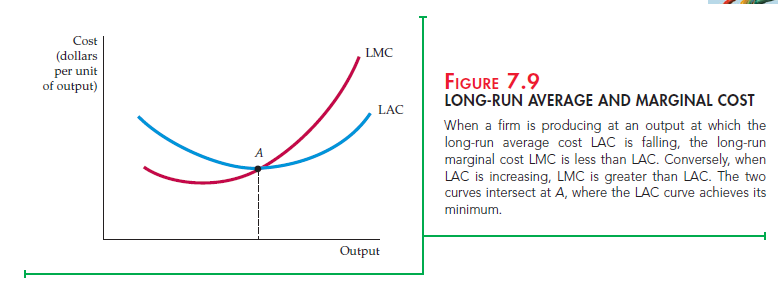
is increased incrementally. LMC lies below the long-run average cost curve when LAC is falling and above it when LAC is rising.10 The two curves intersect at A, where the long-run average cost curve achieves its minimum. In the special case in which LAC is constant, LAC and LMC are equal.
3. Economies and Diseconomies of Scale
As output increases, the firm’s average cost of producing that output is likely to decline, at least to a point. This can happen for the following reasons:
- If the firm operates on a larger scale, workers can specialize in the activities at which they are most productive.
- Scale can provide flexibility. By varying the combination of inputs utilized to produce the firm’s output, managers can organize the production pro- cess more effectively.
- The firm may be able to acquire some production inputs at lower cost because it is buying them in large quantities and can therefore negotiate better prices. The mix of inputs might change with the scale of the firm’s operation if managers take advantage of lower-cost inputs.
At some point, however, it is likely that the average cost of production will begin to increase with output. There are three reasons for this shift:
- At least in the short run, factory space and machinery may make it more difficult for workers to do their jobs effectively.
- Managing a larger firm may become more complex and inefficient as the number of tasks increases.
- The advantages of buying in bulk may have disappeared once certain quantities are reached. At some point, available supplies of key inputs may be limited, pushing their costs up.
To analyze the relationship between the scale of the firm’s operation and the firm’s costs, we need to recognize that when input proportions do change, the firm’s expansion path is no longer a straight line, and the concept of returns to scale no longer applies. Rather, we say that a firm enjoys economies of scale when it can double its output for less than twice the cost. Correspondingly, there are diseconomies of scale when a doubling of output requires more than twice the cost. The term economies of scale includes increasing returns to scale as a special case, but it is more general because it reflects input proportions that change as the firm changes its level of production. In this more general setting, a U-shaped long-run average cost curve characterizes the firm facing economies of scale for relatively low output levels and diseconomies of scale for higher levels.
To see the difference between returns to scale (in which inputs are used in constant proportions as output is increased) and economies of scale (in which input proportions are variable), consider a dairy farm. Milk production is a function of land, equipment, cows, and feed. A dairy farm with 50 cows will use an input mix weighted toward labor and not equipment (i.e., cows are milked by hand). If all inputs were doubled, a farm with 100 cows could double its milk production. The same will be true for the farm with 200 cows, and so forth. In this case, there are constant returns to scale.
Large dairy farms, however, have the option of using milking machines. If a large farm continues milking cows by hand, regardless of the size of the farm, constant returns would continue to apply. However, when the farm moves from
50 to 100 cows, it switches its technology toward the use of machines, and, in the process, is able to reduce its average cost of milk production from 20 cents per gallon to 15 cents per gallon. In this case, there are economies of scale.
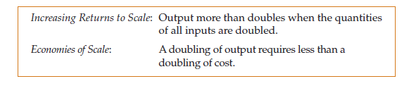
This example illustrates the fact that a firm’s production process can exhibit constant returns to scale, but still have economies of scale as well. Of course, firms can enjoy both increasing returns to scale and economies of scale. It is helpful to compare the two:
Economies of scale are often measured in terms of a cost-output elasticity, EC. EC is the percentage change in the cost of production resulting from a 1-percent increase in output:
![]()
To see how Ec relates to our traditional measures of cost, rewrite equation (7.5) as follows:
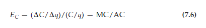
Clearly, Ec is equal to 1 when marginal and average costs are equal. In that case, costs increase proportionately with output, and there are neither economies nor diseconomies of scale (constant returns to scale would apply if input proportions were fixed). When there are economies of scale (when costs increase less than proportionately with output), marginal cost is less than average cost (both are declining) and Ec is less than 1. Finally, when there are diseconomies of scale, marginal cost is greater than average cost and Ec is greater than 1.
4. The Relationship between Short-Run and Long-Run Cost
Figure 7.10 shows the relationship between short-run and long-run cost. Assume that a firm is uncertain about the future demand for its product and is consider- ing three alternative plant sizes. The short-run average cost curves for the three plants are given by SAC1, SAC2, and SAC3. The decision is important because, once built, the firm may not be able to change the plant size for some time.
Figure 7.10 illustrates the case in which there are three possible plant sizes. If the firm expects to produce q0 units of output, then it should build the smallest plant. Its average cost of production would be $8. (If it then decided to produce an output of q1, its short run average cost would still be $8.) However, if it expects to produce q2, the middle-size plant is best. Similarly, with an output of q3, the largest of the three plants would be the most efficient choice.
What is the firm’s long-run average cost curve? In the long run, the firm can change the size of its plant. In doing so, it will always choose the plant that mini- mizes the average cost of production.
The long-run average cost curve is given by the crosshatched portions of the short-run average cost curves because these show the minimum cost of produc- tion for any output level. The long-run average cost curve is the envelope of the short-run average cost curves—it envelops or surrounds the short-run curves.
Now suppose that there are many choices of plant size, each having a differ- ent short-run average cost curve. Again, the long-run average cost curve is the envelope of the short-run curves. In Figure 7.10 it is the curve LAC. Whatever the firm wants to produce, it can choose the plant size (and the mix of capital and labor) that allows it to produce that output at the minimum average cost. The long-run average cost curve exhibits economies of scale initially but exhib- its diseconomies at higher output levels.
To clarify the relationship between short-run and long-run cost curves, consider a firm that wants to produce output q1. If it builds a small plant, the short-run average cost curve SAC1 is relevant. The average cost of production (at B on SAC1) is $8. A small plant is a better choice than a medium-sized plant with an average cost of production of $10 (A on curve SAC2). Point B would therefore become one point on the long-run cost function when only three plant sizes are possible. If plants of other sizes could be built, and if at least one size allowed the firm to produce q1 at less than $8 per unit, then B would no longer be on the long-run cost curve.
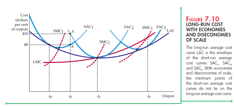
In Figure 7.10, the envelope that would arise if plants of any size could be built is U-shaped. Note, once again, that the LAC curve never lies above any of the short-run average cost curves. Also note that because there are econo- mies and diseconomies of scale in the long run, the points of minimum average cost of the smallest and largest plants do not lie on the long-run average cost curve. For example, a small plant operating at minimum average cost is not effi- cient because a larger plant can take advantage of increasing returns to scale to produce at a lower average cost.
Finally, note that the long-run marginal cost curve LMC is not the envelope of the short-run marginal cost curves. Short-run marginal costs apply to a particu- lar plant; long-run marginal costs apply to all possible plant sizes. Each point on the long-run marginal cost curve is the short-run marginal cost associated with the most cost-efficient plant. Consistent with this relationship, SMC1 intersects LMC in Figure 7.10 at the output level q0 at which SAC1 is tangent to LAC.
Source: Pindyck Robert, Rubinfeld Daniel (2012), Microeconomics, Pearson, 8th edition.
You made some clear points there. I looked on the internet for the topic and found most persons will approve with your blog.