Regression and Correlation of Experimental Data

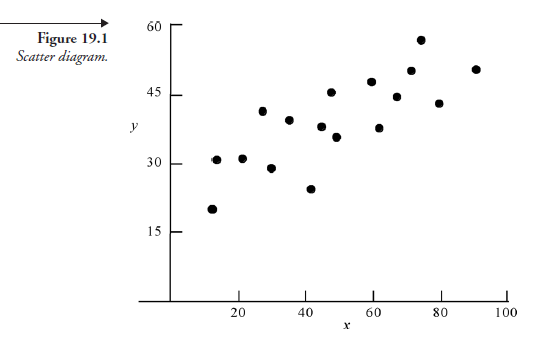
When two sets of variables are associated with any kind of rela­tion, their relation can be represented on a graph as a set of points, each point determined by a pair of corresponding coordi­nates, one from each set. When there is a cause-effect relation, the values of the independent variable are shown on the horizon­tal axis and those of the dependent variable on the vertical axis. Such a graph is known as a scatter diagram (see Figure 19.1) because the points can be scattered without any obvious order. The statistical technique used to develop a mathematical equa­tion representing the relation (if there is one) among the points is known as regression analysis. Depending on how closely such a mathematical equation represents the scatter among all the points, the strength of the relation between the two variables can be determined using a technique known as correlation analysis, the result of which is called the correlation coefficient.

1. Regression Analysis

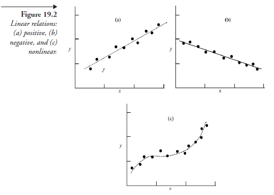
The simplest mathematical relation among several points, each a relation between the independent and the dependent variable, is the equation of a straight line that best fits all the points of the scatter diagram. It is then said that the two variables have a lin­ear relation. Figure 19.2 shows three variations of linear relation: (1) directly (or positively) related, (2) inversely (or negatively) related, and (3) not related, meaning there is no causal relation (though there is an association). We confine ourselves in this book to regression with linear relations only, though there are frequent cases wherein linear regression is not possible. For a study of nonlinear regression, the reader is advised to refer to an advanced book on statistics.

The straight line that best fits all the points of the scatter dia­gram is referred to as the estimated regression line, and the mathe­matical equation describing the line as the estimated regression function. When the function involves only one independent and one dependent variable, the analysis is referred to as a simple lin­ear regression. The most commonly used and the best-suited sim­ple linear regression of experimental results is known as the least- square method. The straight-line equation for this is expressed in the form

where

y = the estimated value of the dependent variable

x = the value of the independent variable

p = the intercept of the y-axis (value of y when x = 0)

a = the change in the dependent variable corresponding to the change in the independent variable (also known as the slope of the line)

In this equation, constants a and p need to be evaluated inde­pendently. The value of a is given by

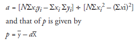
where

xi = the value of the independent variable for the ith observa­tion (i.e., the point in the scatter diagram)

yi = the value of the dependent variable corresponding to x-

X = the mean value of the independent variable

y = the mean value of the dependent variable

N = the total number of observations (i.e., the number of points in the scatter diagram)

The sum of all the squares of the difference between the observed values of the dependent variable, y_i, and the estimated values of the dependent variable, y, meaning the vertical dis­tances of these points from the regression line, will be a mini­mum when the regression line is drawn by this method. That is the reason this method is called the least-square method.

2. Measuring the Goodness of Regression

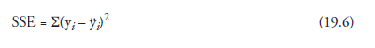
Once the regression line is drawn, it is possible, in principle, to find the y value for any given x value within the extremities; this, indeed, is the purpose of mathematizing the scatter diagram. But the regression line (determined by the regression function) itself is an approximation involving error because all of the points are not located on it but are scattered around it. The error involved is reduced to the least possible by means of regression; the quantity of the error, known as the error sum of squares (SSE), can be expressed as

Suppose the regression were not carried out and the mean of the y values of all the observations (points in the scatter diagram), y, were used as the reference to express the deviation of all the points, we would have what is known as the total sum of squares (SST) about the mean, given by

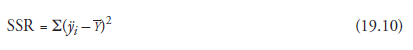
which is also a measure of approximation, and the one with the most possible error in estimation. The benefit of carrying out the regression is that it reduces the possible error from the quan­tity given by SST to that given by SSE. The amount of such a benefit is referred to as the regression sum of squares (SSR), given in quantity by

SSR = SST – SSE                                                                         (19.8)

This relation is one of the most significant theorems of applied statistics. The ratio SSR / SST is a measure of the benefit gained in doing the regression; known as coefficient of determina­tion, it is represented by

This ratio being always less than 1.0, the efficacy of the regres­sion function can also be expressed as a percentage (of the total sum of squares).

Now looking back at (19.8), we want to point out that the value of SSR can be directly evaluated independently of SST and SSE, which can be easily “proved” by a numerical example. Leav­ing this to the reader (if confirmation is desired), the formula required is given below:

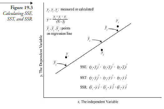
where y is the “estimated” y value of an observation (now to be read on the regression line), and Y is the mean of all the y values as observed. In passing, it may be mentioned that in the fields of business and economics, a correlation with r² = 0.6 or higher is considered satisfactory. In most laboratory experiments, a much higher r² than 0.6 is desirable. Figure 19.3 summarizes the meth­ods for evaluating SSE, SST, and SSR, restricted for demonstra­tion to only three data points.

3. Correlation Coefficient

We remind ourselves that every set of x-y relations is a representa­tive sample of a hypothetical population implied by generalization of the experimental observation. Quite often, the experimenter’s main concern is to know whether or not x and y are related at all, and if they are, to know the strength of their relation. The statisti­cal measure of such strength is known as the correlation coefficient and is given by the value

where r² is the coefficient of determination.

The way it is defined, r can have a “+” or “—” sign, the signifi­cance of which is as follows:

In the equation

y = ax + p,

if the slope (a) is positive, r is taken to be positive, and if (a) is negative, r is taken to be negative. The maximum value that r2 can have being 1.0, r has the range +1 to –1. The correlation coefficient being either +1 or –1 means that the correlation is perfect, in turn meaning that all the points in the scatter diagram are already located on a straight line, a result that is seldom realized in experimental research.

Defining r as above may imply that regression analysis is a prerequisite to get the value of r. This is not so. A sample correlation coefficient can be calculated directly from the experimental observations, shown as the x and y coordinates of the points in the scatter diagram. The formula required is given below:

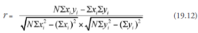
where N is the sample size, that is, the number of observations made with different values of the independent variable, each observation shown as a point in the scatter diagram.

Source: Srinagesh K (2005), The Principles of Experimental Research, Butterworth-Heinemann; 1st edition.