Four-Level Factorial Experiments

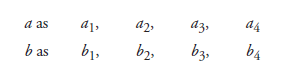
We take the two factors as a and b, and designate the levels of

The sixteen combinations can be lined up as follows:

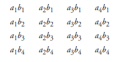
We notice in the above matrix that

1. In the first column, the factor is common, and the only variables are the levels of b: bi, b>2, b3, and b4.
2. In the first row, the factor b₁ is common and the only variables are the levels of a: ai, a2, a3,, and a4.

What the independent variables a and b actually are and how they are regulated and made effective in the experimental setup are of no concern to us. Similarly, what the dependent variable is, how it is recorded, and in what dimensional units do not concern us. What does concern us is having the response—values of the dependent variable, expressed as numbers—correspond to each of the sixteen combinations of the factor levels and analyzing for interpretation relative to the main effects of and interactions, if any, between the two factors.

Table 9.1 lists the corresponding values of the dependent vari­able, alongside the level combinations of the two factors a and b.

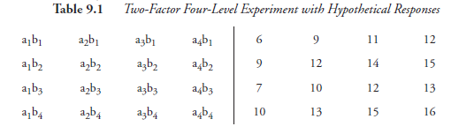
Two-Factor, Four-Level Experiment with Hypothetical Responses

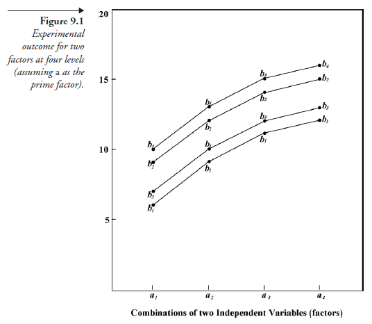
In this table, only whole numbers are used for convenience in demonstration, though in actual experiments, such values are very unlikely. Figure 9.1, in which the same values are presented graphically, provides the following observations:

1. The four levels of factor a are presented on the horizontal scale, also called the x-axis for conve­nience. The locations of points on the x-axis do not represent either the quantities or the units. The distances between points, which are equal in the figure, do not indicate that the levels are at quantitatively equal intervals; they were placed so only for convenience. The quantities and the units thereof depend on the experimenter’s discre­tion. The absence of a factor, for example, may be the first point on the x-axis, not at zero. The sub­sequent points, showing the presence of that fac­tor, do not have to be spaced according to their quantities.
2. The vertical scale (also called the _y-axis for conve­nience) is made to show the numerical values of the dependent variable; this is done strictly to scale.
3. The four levels of factor b do not have a scale of their own. Instead, they appear as four lines, each consisting of three segments: bj—b2, b2—b3, and b3—b^. Each line looks as if it shows the result of a one-factor-at-a-time experiment with a varying and b kept constant. This is not the case.

The above three features will be common to all two-factor, four-level experimental designs.

Now for some observations specific to the numbers in Table 9.1, rendered graphically in Figure 9.1.

Main Effects and Interactions

Looking for the main effects of factors is quite involved here, unlike in Chapter 8, where there was only one “distance” between the “low” and the “high” levels of each factor. In con­trast, here we have three separate distances in series. Referring to the definition of main effect in Chapter 8 and applying it to factor a, we have three, not one, segments of main effect. These are the effects of changing a from level 1 to level 2, from level 2 to level 3, and from level 3 to level 4. Also, with only two levels of fac­tors, it was possible in Chapter 8 to assign a “—” to the low and a “+” to the high levels of factors. Further, taking advantage of the “—1” and “+1” symbolism, analyzing the values of the dependent variable could be done “mechanically” (see Tables 8.8 to 8.11). That advantage is not available for an analysis in which the fac­tors are dealt with at more than two levels.

The four lines of each segment level are parallel to each other. In terms of numbers, we may say the distance between any two levels of factor b (which is a measure of the improvement attrib­utable to factor b) is the same at different levels of factor a. In other words, factor b is uniformly effective at different levels of a. This is a situation of factor b improving (supplementing, we may say) the effect of a, but not interacting with it. Thus, the four lines, each corresponding to a level of factor b, signal the condi­tion of no interaction between the two factors within the range of the factor levels used in the experiment.

As mentioned earlier, it is likely and desirable that either a or b can be identified as the prime factor. If a can be so identified, it is desirable to locate it on the x-axis, as is done in Figure 9.1. Suppose in the experiment we are presently discussing that b is the prime factor. In such a situation, the same data as we now have in Table 9.1 can be rearranged as shown in Figure 9.2.

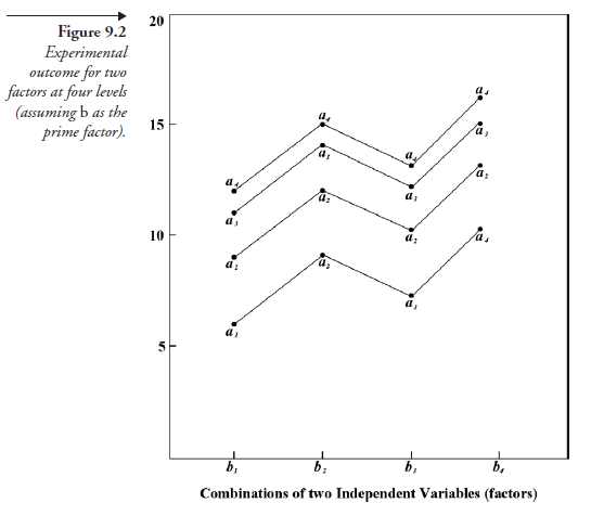
Comparing this figure with Figure 9.1, we notice that the four lines, each corresponding to a level of a, are again parallel to each other, though the shapes of all the lines in Figure 9.2 are different from those in Figure 9.1. We may thus summarize that whatever the shape of the lines corresponding to different levels of the sec­ond factor, the lines being parallel is the criterion test for no interaction between the two factors. Now, though it is desirable to identify one of the two factors as the prime factor, it may often be impossible, even presumptuous, to do so. The mere fact of the lines being parallel should be an adequate test for no interaction.

Source: Srinagesh K (2005), The Principles of Experimental Research, Butterworth-Heinemann; 1st edition.