Testing of Hypothesis in Experimental Research

Testing of statistical hypothesis has several applications, almost wherever statistics is applicable. In this book, however, we shall confine the discussion to experimental research, considering only one obvious and hypothetical case of application; this will show the way to other possible applications with minor modifications as required.

Let us imagine that an experiment has been conducted previ­ously. If that experiment is replicated elsewhere at a later date, with no change in the independent variables, instrumentation, and material involved, we expect the value of the dependent vari­able to be the same as in the previous experiment. Suppose the value of the dependent variable was previously thirty. We further assume that thirty was an ideal minimum number to confirm a theory. If the corresponding value in the present experiment comes out to be twenty-nine, should the theory be rejected? In this situation, thirty, the number we made reference to, is in effect, the hypothesis. And, the statistical consideration and the procedures involved in rejecting or accepting the theory in ques­tion constitute the testing of the hypothesis.

Example:

This experiment consists of a student trying to confirm the results of a previous Ph.D. dissertation. The professor who has guided the Ph.D. work has recently come to doubt the result of that work; the reputation of the previous student (hence, his own) is being questioned. The Ph.D. work is supposed to have confirmed a theory developed by the professor. The confirmation depended on a certain minimum number, which was the out­come, as the dependent variable, of the experiment done with the specific independent variables in the experiment. There is a state­ment in the Ph.D. thesis to the effect that the mean of a large number of replications gave the value of the dependent variable as 53.2, with a standard deviation of 1.4. Thus, 53.2 is the num­ber required to confirm the theory.

Another student of the same professor is the present experi­menter. As far as this student can manage, he has reproduced the conditions of the Ph.D. experiments. His numbers are 51.5, 54.3, 53.1, 52.0, 53.6, 52.7, and 51.9 (we will suppress the units, millivolts, for convenience.) The mean of these readings, 52.7, is less than 53.2, the minimum expected. The present student is inclined to reject the previous confirmation of the theory, to that extent claiming credit for himself. The professor, having previ­ously used the statistical methods, is not in such a hurry. Testing of the hypothesis starts here; the number 53.2 is at the core of the hypothesis.

In the following hypothesis, μ0 represents 53.2, and μ1 represents the mean of the values of the dependent variable from the current experiments. We state the hypothesis for this case somewhat differently from how we did before.

The null hypothesis, H0: μ1 ≥ μ0 (53.2), means, if μ1 is equal to or greater than 53.2, there is no need to doubt the previous experiment; action is not necessary.

The alternate hypothesis, Ha: μ1 < μ0(52.3), means, if μ1 is less than 53.2, doubt is valid, and action is necessary.

“Action” in both cases constitutes rejecting the theory based on the confirmation by previous experiment.

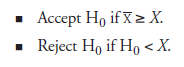
The fact that the mean of the present seven values is less than 53.2 is not statistically important because this is the sample mean, X (not the population mean), and that too calculated from a small sample. Further, dealing with probability, not certainty, we need to know how much lower than 53.2 the value of X can be to safely reject H₀. This situation calls for a criterion value to be compared with X; we will designate such a value as Now the decision rules can be formulated as

The next steps are

1. To get a more dependable X, meaning more repli­-cations, preferably more than thirty
2. To find by statistical analysis a “reasonable” value of X

Assuming that the present experimenter is engaged in per­forming more replications, together amounting to 32(N), we will attend to the statistical part, step (2), below:

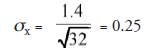
Applying the Central Limit Theorem (see Chapter 17), we know that the population mean, μ0, is given by the mean of (many) X values and that the standard deviation of the X’s, σx, is given by , in which σ is the population mean.

In our case

Now the probability of rejecting H0 needs to be addressed. Being conscious that his reputation is at stake, the professor is likely to be very conservative. We assume that his decision is to allow only a 1 percent chance of ejecting H0, meaning α = 0.01. Using the notation of the standard normal distribution (see Chapter 17), we can now write the value of X:

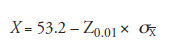
Going to the table of standard normal distribution, we find the z value for the probability of 0.5 – 0.01 = 0.49 to be 2.33. Substituting 2.33 for Z0.01 and 0.25 for σX, we can find X.

X = 53.2 – 2.33 × 0.25 = 52.6.

Now we can state the decision in terms of concrete numbers:

Accept H0 (action is not necessary) if X ≥ 52.6. Reject H0 (action is necessary) if X < 52.6. “Action,” in both cases, constitutes disowning the previous experiment, hence, rejecting the theory based on that experiment. The mean of the value of the dependent variable, X, from thirty-two replications to be performed by the present experimenter, serves as the key in this decision.

Source: Srinagesh K (2005), The Principles of Experimental Research, Butterworth-Heinemann; 1st edition.