Statistical Tests in the Research

In this section we explore the general context in which researchers carry out statistical tests. We define the essential concepts involved and outline the gene­ral steps followed when using this type of test.

1. Inference and Statistics

Inference has a very important place in management research. Conclusions or generalizations often have to be established on the basis of observations or results, and in some cases statistics can add to their precision. As inference is often at the heart of the reasoning by which the statistician generalizes from a sample to a population, the branch of statistics devoted to this type of approach is called inferential statistics. The goal of inferential statistics is to evaluate hypotheses through information collected from a selected sample. Statistical tests are thus at the very core of inferential statistics.

2. Research Hypotheses

Research hypotheses are unproven statements about a research field. They may be based on existing theoretical material, previous empirical results, or even personal impressions or simple conjecture. For instance, one of Robinson and Pearce’s (1983: 201) research hypotheses was ‘Banks engaging in formal plan­ning will have a significantly higher mean performance ranking than non­formal planning banks from 1977 and 1979’. If researchers want to use statistical tests to prove a research hypothesis, they must first translate the hypothesis into a statistical hypothesis.

3. Statistical Hypotheses

A statistical hypothesis is a quantified statement about the characteristics of a population. More precisely, it describes the distribution of one or more random variables. It might describe the parameters of a given distribution, or a proba­bility distribution of an observed population.

A statistical hypothesis is generally presented in two parts: the null hypothesis and the alternative or contrary hypothesis. These two hypotheses are incompatible. They describe two complementary states. The null hypothesis describes a situa­tion in which there is no major shift from the status quo, or there is an absence of difference between parameters. The alternative hypothesis – that there is a major shift from the status quo, or that there is a difference between parameters – is generally the hypothesis the researcher wishes to establish. In this case the alter­native hypothesis corresponds to the research hypothesis – the researcher believes it to be true (Sincich, 1996). The researcher’s goal is then to disprove the null hypothesis in favor of the alternative hypothesis (Sincich, 1996; Zikmund, 1994).

The null hypothesis is generally marked H₀ and the alternative (or contrary) hypothesis H₁ or H_a. It is important to bear in mind that statistical tests are designed to refute and not to confirm hypotheses. In other words, these tests do not aim to prove hypotheses, and do not have the capacity to do so. They can only show that the level of probability is too low for a given statement to be accepted (Kanji, 1993). For this reason, statistical hypotheses are normally formu­lated so that the alternative hypothesis H₁ corresponds to the research hypo­thesis one is trying to establish. In this way, rather than attempting to prove that this hypothesis is correct, the goal becomes to reject the null hypothesis.

4. Statistical Tests

Statistical tests are used to assess the validity of statistical hypotheses. They are carried out on data collected from a representative sample of the studied popu­lation. A statistical test should lead to rejecting or accepting an initial hypothesis: in most cases the null hypothesis.

Statistical tests generally fall into one of two categories: parametric tests and non-parametric tests.

Statistical tests were first used in the experimental sciences and in manage­ment research. For instance, the Student test was designed by William Sealy Gosset (who was known as ‘Student’), when working with Guinness breweries. But the mathematical theory of statistical tests was developed by Jerzy Neyman and Egon Shape Pearson. These two authors also stressed the importance of considering not only the null hypothesis, but also the alternative hypothesis (Lehmann, 1991).

In a statistical test focusing on one parameter of a population, for instance its mean or variance, if the null hypothesis H₀ states one value for the parameter, the alternative hypothesis H₁ would state that the parameter is different from this specific value.

In a statistical test focusing on the probability distribution of a population, if the null hypothesis H₀ states that the population follows a specific distribution, for example a normal distribution, the alternative hypothesis H₁ would state that the population does not follow this specific distribution.

4.1. A single population

The number of populations being considered will influence the form of the statistical test. If a single population is observed, the test may compare a para­meter 0 of the population to a given value 0_O.

For example, Robinson and Pearce (1983: 201) hypothesized that companies with a formal planning policy will perform better than companies without such a policy. In this case the statistical test used would be a one-tail test to the right (a right-tail test). If the hypothesis had suggested that inferior performance resulted from formal planning, a one-tail test to the left (a left-tail test) would be used. If, however, the two authors had simply hypothesized that formal planning would lead to a difference in performance, without specifying in which direction, a two-tail test would have been appropriate. These three alter­native hypotheses would be formulated as follows:

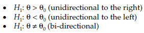
where 0 corresponds to the performance of companies with a formal planning policy, and 0₀ to the performance of companies without such a policy.

Sometimes, the null hypothesis can also be expressed as an inequation. This gives the following hypotheses systems:

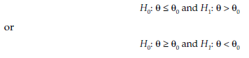
In these cases, the symbols ‘<‘ (less than or equal to) and ‘>’ (greater than or equal to) are used in formulating the null hypothesis H₀ in order to cover all cases in which the alternative hypothesis H_P is not valid.

However, the general convention is to express H₀ as an equation. The rea­soning behind this convention is the following: if the alternative hypothesis is stated as an inequation, for instance Hp θ > θ₀, then every test leading to a rejec­tion of the null hypothesis H₀: θ = θ₀ and therefore to the acceptance of the alter­native hypothesis Hp θ > θ₀, would also lead to the rejection of every hypothesis H₀: θ = θ_i, for every θ_i inferior to θ₀. In other words, H₀: θ = θ₀ represents the most unfavorable situation possible (from the researcher’s point of view) if the alter­native hypothesis Hp θ>θ₀ turned out to be incorrect. For this reason, express­ing the null hypothesis as an equation covers all possible situations.

4.2. Two populations

When a statistical test focuses on the parameters of two populations, the goal is to find out whether the two populations described by a specific parameter are different. If θ1 and θ₂ represent the parameters of the two populations, the null hypothesis predicts the equality of these two parameters:

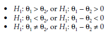
The alternative hypothesis may be expressed in three different ways:

4.3. More than two populations

A statistical test on k populations aims to determine if these populations differ on a specific parameter. θ1 θ₂, … , θ_k are the k parameters describing the k popu­lations being compared. The null hypothesis would be that the k parameters are identical:

The alternative hypothesis would then be formulated as follows:

This means that the null hypothesis will be rejected in favor of the alterna­tive hypothesis if the value for any single parameter is found to be different from that of another.

5. Risk of Error

Statistical tests are used to give an indication as to what decision to make – for instance, whether to reject or not to reject the null hypothesis H₀. As this deci­sion is, in most research situations, based on partial information only, derived from observations made of a sample of the population, a margin of error is involved (Sincich, 1996; Zikmund, 1994). A distinction is made between two types of error in statistical tests: error of the first type, or Type I error (a), and error of the second type, or Type II error (P).

5.1. Type I and Type II error

By observing the sample group, a researcher may be lead mistakenly to reject the null hypothesis – when in fact the population actually fulfills the conditions of this hypothesis. Type I error (a) measures the probability of rejecting the null hypothesis when it is in fact true. Conversely, a researcher’s observations of a sample may not allow the null hypothesis to be rejected, when in fact the popula­tion actually satisfies the conditions of the alternative hypothesis. Type II error (P) measures the probability of not rejecting the null hypothesis when it is in fact false.

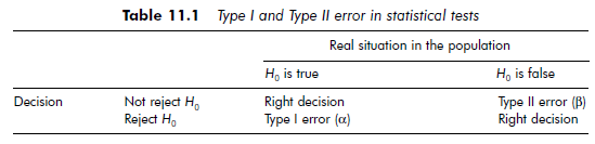
As the null hypothesis may be true or false and the researcher may reject it or not reject it, there are only four possible and mutually exclusive outcomes of a statistical test. These are presented in Table 11.1.

Only two of the four cases in Table 11.1 involve an error. Type I error can only appear if the null hypothesis is rejected. In the same way, Type II error is only possible if the null hypothesis is not rejected. The two types of error can never be present at the same time.

It is tempting to choose a minimal value for Type I error a. Unfortunately, decreasing this value increases Type II error, and vice versa. The only way to minimize both a and P is to use a larger sample (Sincich, 1996). Otherwise, a compromise must be sought between a and P, for example by measuring the power of the test.

When using statistical tests, it is preferable not to speak of accepting the null hypothesis, but rather of not rejecting it. This semantic nuance is important: if the aim of the test was to accept H₀, the validity of its conclusion would be measured by Type II error P – the probability of not rejecting the null hypothesis when it is false. However, the value of P is not constant. It varies depending on the specific values of the parameter, and is very difficult to calculate in most statistical tests (Sincich, 1996). Because of the difficulty of calculating P, making a decision based upon the power of the test or the effectiveness curve can be tricky.

There is actually another, more practical solution; to choose a null hypothesis in which a possible Type I error a would be much more serious than a Type II
error P. For example, to prove a suspect guilty or innocent, it may be preferable to choose as the null hypothesis ‘the suspect is innocent’ and as the alternative hypothesis ‘the suspect is guilty’. Most people would probably agree that in this case, a Type I error (convicting someone who is innocent) is more serious than a Type II error (releasing someone who is guilty). In such a context, the researcher may be content to minimize the Type I error a.

5.2. Significance level

Before carrying out a test, a researcher can determine what level of Type I error will be acceptable. This is called the significance level of a statistical test.

A significance level is a probability threshold. A significance level of 5 per cent or 1 per cent is common in management research. In determining a significance level, a researcher is saying that if Type I error – the probability of wrongly rejecting a null hypothesis – is found to be greater than this level, it will be considered significant enough to prevent the null hypothesis H₀ from being rejected.

In management research, significance level is commonly marked with aste­risks. An example is the notation system employed by Horwitch and Thietart (1987): p < 0.10*; p < 0.05**; p < 0.01***; p < 0.001****, where one asterisk corres­ponds to results with a 10 per cent significance level, two asterisks 5 per cent, three asterisks 1 per cent and four asterisks 0.1 per cent (that is, one in one thousand). If no asterisk is present, it means the results are not significant.

6. To Reject or not to Reject?

6.1. Statistic X

The decision to reject or not to reject the null hypothesis H₀ is based on the value of a relevant statistic – which we refer to as a statistic X. A statistic X is a random variable, appropriate to the null hypothesis H₀. It is calculated from data collected from one or more representative samples from one or more popu­lations (Kanji, 1993). A statistic X may be quite simple, such as the mean or the variance, or it may be a complex function of these and other parameters. We will look at different examples later in this chapter.

A good statistic should present three characteristics (Kanji, 1993):

1. It must behave differently according to whether H₀ is true (and H₁ false) or vice versa.
2. Its probability distribution when H₀ is true must be known and calculable.
3. Tables defining this probability distribution must be available.

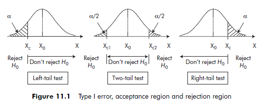
6.2. Rejection region, acceptance region, and critical value

The set of values of the statistic X that lead to rejecting the null hypothesis is called the rejection region (or the critical region). The complementary region is called the acceptance region (or, more accurately, the non-rejection region). The value representing the limit of the rejection region is called the critical value. In a one-tail test, there is only one critical value X_c, while in a two-tail test, there are two; X_c1 and X_c2. The acceptance region and the rejection region are both dependant on Type I error a, since a is the probability of rejecting H₀ when it is actually true, and 1-a is the probability of not rejecting H₀ when it is true. This relationship is illustrated by Figure 11.1.

Rules for rejecting or not rejecting the null hypothesis

• For a left-tail test, the null hypothesis is rejected for any value of the statistic X lower than the critical value X_c. The rejection region therefore comprises the values of X that are ‘too low’.
• For a two-tail test, the null hypothesis H₀ is rejected for values of the statistic X that are either less than the critical value X_c1 or greater than the critical value X_c2. The rejection region here comprises the values of X that are either ‘too low’ or ‘too high’.
• Finally, for a right-tail test, the null hypothesis is rejected for any value of the statistic X greater than the critical value X_c. The rejection region in this case comprises the values of X that are ‘too high’.

6.3. P-value

Most statistical analysis software programs provide one very useful piece of information, the p value (also called the observed significance level). The p value is the probability, if the null hypothesis were true, of obtaining a value of X as extreme as the one found for a sample. The null hypothesis H₀ will be rejected if the p value is lower than the pre-determined significance level a (Sincich, 1996).

It is becoming increasingly common to state the p value of a statistical test in published research articles (for instance Horwitch and Thietart, 1987). Readers can then compare the p value with different significance levels and see for themselves if the null hypothesis should be rejected or not. The p value also locates the statistic X in relation to the critical region (Kanji, 1993). For instance, if some data indicates that the null hypothesis H₀ should not be rejected, the p value may be just below the chosen significance level; while if the data provides solid reasons to reject the null hypothesis, the p value would be noticeably lower than the significance level.

7. Defining a Statistical Test – Step-by-Step

Statistical tests on samples generally follow the following method.

In practice, the task is much easier than this. Most statistical analysis software (SAS, SPSS, etc.) determine the statistic X appropriate to the chosen test, calculate its value, and indicate the p value of the test. Some programs, such as Statgraphics, will even go one step further and suggest whether the null hypothesis should be rejected or not according to the significance level fixed by the researcher.

The major difficulty researchers face, though, is to choose the right test. The two following sections provide guidelines for making this choice, first looking at parametric and then at non-parametric tests. The tests are presented in terms of research aims and the research question, and the conditions attached to the application of each test are enumerated.

Source: Thietart Raymond-Alain et al. (2001), Doing Management Research: A Comprehensive Guide, SAGE Publications Ltd; 1 edition.