Parametric Tests in the Research

1. Tests on Means

1.1. Comparing the mean m of a sample to a reference value μ0 when the variance σ₂ of the population is known

Research question Does the mean m, calculated from a sample taken from a population with a known variance of σ₂, differ significantly from a hypothetical mean μ₀?

Application conditions

• The variance σ₂ of the population is known (this is a very rare case!) but the mean m is not known (the hypothesis suggests it equals m ₀).
• A random sample is used, containing n independent observations
• The size n of the sample should be greater than 5, unless the population fol­lows a normal distribution, in which case the size has no importance. Actually, this size condition is to guarantee the mean of the sample follows a normal distribution (Sincich, 1996).

Hypotheses

The null hypothesis to be tested is H₀: μ = μ₀,

the alternative hypothesis is H1: μ # μ₀ (for a two-tail test)

or Hp μ < μ₀ (for a left-tail test)

or Hp μ # μ₀ (for a right-tail test)

Statistic The statistic calculated is

It follows a standard normal distribution (mean = 0 and standard deviation = 1). This is called a z test or a z statistic.

Interpreting the test

• In a two-tail test, H₀ will be rejected if Z < – Z_a/2 or Z > Z_a/2
• in a left-tail test, H₀ will be rejected if Z < – Z_a
• in a right-tail test, H₀ will be rejected if Z > Z_a
  where a is the defined significance level (or Type I error), and Z_a and Z_a/2 are the normal distribution values that can be found in the appropriate tables.

1.2. Comparing the mean m of a sample to a reference value when μ0 when the variance σ₂ of the population is nknown

Research question Does the mean m, calculated from a sample taken from a population with an unknown variance σ², differ significantly from a hypothe­tical mean μ₀?

Application conditions

• The variance σ² of the population is not known and has to be estimated from the sample. The mean m is also unknown (the hypothesis suggests it equals m ₀).

• A random sample is used, containing n independent observations.
• The size n of the sample is greater than 30, unless the population follows a normal distribution, in which case the size has no importance.

Hypotheses

Null hypothesis, H₀: μ = μ₀,

the alternative hypothesis is H1: μ # μ₀ (for a two-tail test)

or Hp μ < μ₀ (for a left-tail test)

or Hp μ # μ₀ (for a right-tail test)

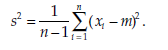
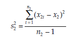
Statistic The unknown variance (o₂) of the population is estimated from the sample, with n – 1 degrees of freedom, using the formula

The statistic calculated is

It follows Student’s distribution with n – 1 degrees of freedom, and is called a t test or a t statistic.

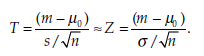
Interpreting the test When n is large, that is, greater than 30, this statistic approximates a normal distribution. In other words:

The decision to reject or not to reject the null hypothesis can therefore be made by comparing the calculated statistic T to the normal distribution values. We recall that the decision-making rules for a standard normal distribution are:

• in a two-tail test, H₀ will be rejected if Z <- Z_a/2 or Z > Z_a/2
• in a left-tail test, H₀ will be rejected if Z <- Z_a
• in a right-tail test, H₀ will be rejected if Z > Z_a.

where a is the significance level (or Type I error) and Z_a and Z_a/2 are normal distribution values, which can be found in the appropriate tables.

But for smaller values of n, that is, lower than 30, the Student distribution (at n – 1 degrees of freedom) cannot be replaced by a normal distribution. The decision rules then become the following:

• In a two-tail test, H₀ will be rejected if T <- T_{a/2; n} _ ₁ or T > T_{a/2; n} _ ₁
• in a left-tail test, H₀ will be rejected if T <- T_a. _n _ ₁
• in a right-tail test, H₀ will be rejected if T > T_a. _n _ ₁.

Example: Comparing a mean to a given value (variance is unknown)

This time, the sample is much larger, containing 144 observations. The mean found in this sample is again m _ 493. The estimated standard deviation is s _ 46.891. Is it still possible to accept a mean in the population p₀ _ 500, if we adopt a significance level a of 5 per cent?

The relatively large size of the sample (n _ 144, and so is greater than 30) justifies the approximation of the statistic T to a normal distribution. Thus

which gives -1.79. The tables provide values of Z_0.025 _ 1.96 and Z_0.05 _ 1.64.

Two-tail test: As – Z_a/₂ < T < Z_a/₂ ( -1.96 < -1.79 < 1.96), the null hypothesis, stat­ing that the mean of the population equals 500 (p = 500), cannot be rejected.

Left-tail test: as T < – Z_a (-1.79 < -1.64), the null hypothesis is rejected, to the benefit of the alternative hypothesis, according to which the mean in the population is less than 500 (p < 500).

Right-tail test: as T < Z_a (-1.79 < 1.64), the null hypothesis cannot be rejected.

As mentioned above, the major difficulty researchers face when carrying out comparison tests is to choose the appropriate test to prove their research hypo­thesis. To illustrate this, in the following example we present the results obtained by using proprietary computer software to analyze the above situation. For this example we will use the statistical analysis program, Statgraphics, although other software programs provide similar information.

The software carries out all the calculations, and even indicates the decision to make (to reject the null hypothesis or not) on the basis of the statistic T and the significance level a set by the researcher. In addition, it provides the p value, or the observed significance level. We have already mentioned the importance of the p value, which can provide more detailed information, and so refine the decision. In the first test (two-tail test), the null hypothesis is not rejected for a significance level of 5 per cent, but it would have been rejected if the Type I error risk had been 10 per cent. The p value (0.0753462) is greater than 5 per cent but less than 10 per cent. In the second test (left-tail test), the null hypothesis is rejected for a significance level of 5 per cent, while it would not have been rejected for a significance level of 1 per cent. The p value (0.0376731) is less than 5 per cent but greater than 1 per cent. Finally, in the last test (right-tail test), examining the p value (0.962327) suggests that there are good reasons for not rejecting the null hypothesis, as it is well above any acceptable significance level.

1.3. Comparing the difference of two means to a given value, when the variance of the two populations is known

Research question Is the difference between the two means p₁ and p₂ of two populations of known variances o2 and o2 significantly different from a given value D₀ (for instance zero)?

Application conditions

• The variances o2 and o2 of the two populations are known. The means p₁ and p₂ are unknown.
• Both samples are random and contain n₁ and n₂ independent observations respectively.
• Either the mean for each population follows a normal distribution, or the size of each sample is greater than 5.

Hypotheses

Null hypothesis, H₀: μ₁ – μ₂ = D₀,

the alternative hypothesis is H1: μ₁ – μ₂ # D₀ (for a two-tail test)

or Hp μ₁ – μ₂ < D₀ (for a left-tail test)

or Hp μ₁ – μ₂ > D₀ (for a right-tail test)

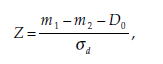
Statistic

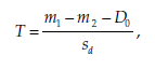
The statistic calculated is

x1i = the value of variable X for observation i in population 1,
x2i = the value of variable X for observation i in population 2,

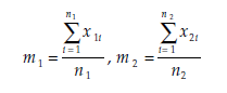
and

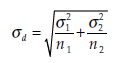
is the standard deviation of the difference (m₁-m₂).

Z follows a standard normal distribution.

Interpreting the test The decision rules are the following:

• In a two-tail test, H₀ will be rejected if Z < -Z_a/2 or Z > Z_a/2
• in a left-tail test, H₀ will be rejected if Z < – Z_a
• in a right-tail test, H₀ will be rejected if Z > Z_a.

1.4. Comparing the difference of two means to a given value, when the two populations have the same variance, but its exact value is unknown

Research question Is the difference between the two means m₁ and m₂ of two populations that have the same unknown variance σ² significantly different from a given value D₀ (for instance zero)?

Application conditions

• The two populations have the same unknown variance (σ²). The two means μ₁ and μ₂ are not known.
• Both samples are random and contain n₁ and n₂ independent observations respectively.
• Either the mean for each population follows a normal distribution, or the size of each sample is greater than 30.
• The hypothesis of equality of the variances is verified (see Section 3.2 of this chapter).

Hypotheses

Null hypothesis, H₀: μ₁ – μ₂ = D₀,

the alternative hypothesis is H1: μ₁ – μ₂ # D₀ (for a two-tail test)

or Hp μ₁ – μ₂ < D₀ (for a left-tail test)

or Hp μ₁ – μ₂ > D₀ (for a right-tail test)

Statistic

The statistic calculated is:

x_1i = the value of the observed variable X for observation i in population 1,

x_2i = the value of the observed variable X for observation i in population 2,

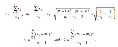
This statistic follows Student’s t distribution with n₁ + n₂ – 2 degrees of freedom.

Interpreting the test The decision rules are the following:

• in a two-tail test, H₀ will be rejected if T <- T_{a/2; n1} + _n2 _ ₂ or T > T_{a/2; n1} + _n2 _ ₂
• in a left-tail test, H₀ will be rejected if T <- T _n1+_n2 _ ₂
• in a right-tail test, H₀ will be rejected if T > T _n1 + _n2 _ ₂.

When the sample size is sufficiently large (that is, n₁ > 30 and n₂ > 30), the distribution of the statistic T approximates a normal distribution, in which case

The decision to reject or not to reject the null hypothesis can then be made by comparing the calculated statistic T to the normal distribution. In this case, the following decision rules should apply:

• In a two-tail test, H₀ will be rejected if T <- Z_a/2 or Z > Z_a/2
• in a left-tail test, H₀ will be rejected if T <- Z_a
• in a right-tail test, H₀ will be rejected if T > Z_a.

1.5. Comparing two means, when the variances of the populations are unknown and differ

Research question Do the two means μ₁ and μ₂ of two populations of unknown variances and differ significantly from each other?

Application conditions

• The variances σ1 and σ2 of the two populations are unknown and different. The means μ₁ and μ₂ are unknown.
• Both samples are random and contain n₁ and n₂ independent observations respectively.
• For both populations, the mean follows a normal distribution.
• The two samples are of practically the same size.
• At least one of the samples contains fewer than 20 elements.
• The hypothesis of the inequality of variances is fulfilled (see Section 3.2 of this chapter).

Hypotheses

Null hypothesis, H₀: μ₁ = μ₂,

the alternative hypothesis is H1: μ₁ # μ₂ (for a two-tail test)

or Hp μ₁ < μ₂ (for a left-tail test)

or Hp μ₁ > μ₂ (for a right-tail test)

Statistic Using the same notations as in Section 1.4 of this chapter, the statistic calculated is:

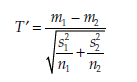
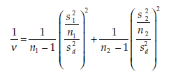
This statistic T’ is called an Aspin-Welch test. It approximates a Student T distribution in which the number of degrees of freedom v is the closest integer value to the result of the following formula:

Interpreting the test The decision rules then become the following:

• in a two-tail test, H₀ will be rejected if T’ <- T_a/2; v or T’ > T_a/2; v
• in a left-tail test, H₀ will be rejected if T’ <- T_{a; v}
• in a right-tail test, H₀ will be rejected if T > T_a. _v.

1.6. Comparing k means (μ_k): analysis of variance

Research question Do k means, m₁, m₂… , m_k observed on k samples differ sig­nificantly from each other?

This question is answered through an analysis of variance (Anova).

Application conditions

• All k samples are random and contain n₁, n₂… n_k independent observations.
• For all k populations, the mean approximates a normal distribution with the same, unknown, variance (σ²).

Hypotheses

Null hypothesis, H₀: π₁ = π₂ = … = π_k,

alternative hypothesis, Hp the values of πi (i = 1, 2, … , k) are not all identical. This means that one single different value would be enough to reject the null hypothesis, thus validating the alternative hypothesis.

Statistic The statistic calculated is

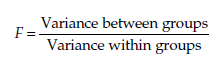
The statistic F follows a Fisher distribution with k – 1 and n – k degrees of free­dom, where n is the total number of observations.

Interpreting the test The decision rule is the following:

H₀ will be rejected if F > F_k _ _{1; n} _ _k.

The analysis of variance (Anova) can be generalized to the comparison of the mean profiles of k groups according to j variables Xj. This analysis is called a Manova, which stands for ‘multivariate analysis of variance’. Like the Anova, the test used is Fisher’s F test, and the decision rules are the same.

1.7. Comparing k means (μ_k): multiple comparisons

Research question Of k means m₁, m₂… , m_k observed on k samples, which if any differ significantly?

The least significant difference test, or LSD, is used in the context of an Anova when examination of the ratio F leads to the rejection of the null hypo­thesis H₀ of the equality of means, and when more than two groups are present. In this situation, a classic analysis of variance will only furnish global informa­tion, without indicating which means differ. LSD tests, such as the Scheffe, Tukey, or Duncan tests, compare the groups two by two. These tests are all included in the major statistical analysis computer programs.

Application conditions

• All k samples are random and contain n₁, n₂… n_k independent observations.
• For all k populations, the mean approximates a normal distribution with the same, unknown, variance (o²).

Hypotheses

Null hypothesis, H₀: π₁ = π₂ = … = π_k,

alternative hypothesis, H₁: the values of π_i (i = 1, 2, … , k) are not all identical. This means that one single different value would be enough to reject the null hypothesis, thus validating the alternative hypothesis.

 Statistic

The statistic calculated is

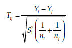
where Y_i. is the mean of Group i, Y. the mean of group j, n_i the number of observations of group i, nj the number of observations of group j, and S2 the esti­mation of the variance within each group. This statistic T. follows a Student distribution with n – k degrees of freedom, where n is the total number of obser­vations. This signifies that the mean of all the two-by-two combinations of the k groups will be compared.

Interpreting the test The decision rule is the following:

H₀ will be rejected if one Tj is greater than T_{a/2; n} __k. When T_ij > T_{a/2; n} _ _k, the dif­ference between the means Y_i. and Y- of the two groups i and j in question is judged to be significant.

1.8. Comparing k means (μk): analysis of covariance

Research question Do k means m₁, m₂… , m_k observed on k samples differ sig­nificantly from each other?

Analysis of covariance permits the differences between the means of dif­ferent groups to be tested, taking the influence of one or more metric vari­ables, Xj called concomitants, into account. This essentially involves carrying out a linear regression to explain the means in terms of the X- concomitant variables, and then using an analysis of variance to examine any differences between groups that are not explained by the linear regression. Analysis of covariance is therefore a method of comparing two or more means. Natur­ally, if the regression coefficients associated with the explicative concomitant metric variables are not significant, an analysis of variance will have to be used instead.

Application conditions

• All k samples are random and contain n₁, n₂… n_k independent observations.
• For all k populations, the mean approximates a normal distribution with the same, unknown, variance (o²).
• The choice of structure of the k groups should not determine the values of the concomitant metric variables.

Hypotheses

Null hypothesis, H₀: π₁ = π₂ = … = π_k,

alternative hypothesis, Hp the values of π_i (i = 1, 2, … , k) are not all identical. This means that one single different value would be enough to reject the null hypothesis, thus validating the alternative hypothesis.

Statistic

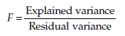
where the explained variance is the estimation made from the sample of the variance between the groups, and the residual variance is the estimation of the variance of the residues. This statistic F follows a Fisher distribution, with k – 1 and n – k – 1 degrees of freedom, n being the total number of observations.

Interpreting the test The decision rule is the following:

H₀ will be rejected if F > F_k _ _{1; n} __k _ ₁. The statistic F and the observed significance level are automatically calculated by statistical analysis software.

The analysis of covariance (Ancova) can be generalized to the comparison of the mean profiles of k groups according to j variables X. This is called a Mancova, for ‘multivariate analysis of covariance’. The test used (that is, Fisher’s F test) and the decision rules remain the same.

1.9. Comparing two series of measurements: the hotelling T² test

Research question Do the mean profiles of two series of k measurements (m₁, m₂ … , m_k) and (m’_v m’₂, … , mf), observed for two samples, differ significantly from each other?

The Hotelling T² test is used to compare any two matrices or vectors, particu­larly correlation matrices, variance or covariance matrices, or mean-value vectors.

Application conditions

• The two samples are random and contain n₁ and n₂ independent observa­tions respectively.
• The different measurements are independent and present a normal, multi­variate distribution.

Hypotheses

Null hypothesis, H₀: the two series of measurements present the same profile, alternative hypothesis, H₁: the two series of measurements present different profiles.

Statistic

The statistic calculated is

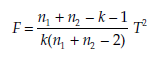
where T² is Hotelling’s T², k the number of variables, and n₁ and n₂ are the number of observations in the first and second sample.

The statistic F follows a Fisher distribution with k and n₁ + n₂ – k – 1 degrees of freedom.

Interpreting the test The decision rule is the following:

^H0 will be rejected if  ^F > ^Fk _ 1; n1 + n2 – k – 1.

2. Proportion Tests

2.1. Comparing a proportion or a percentage to a reference value π₀: binomial test

Research question Does the proportion p, calculated on a sample, differ signi­ficantly from a hypothetical proportion π₀?

Application conditions

• The sample is random and contains n independent observations.
• The distribution of the proportion in the population is binomial.
• The size of the sample is relatively large (greater than 30).

Hypotheses

Null hypothesis, H₀: π = π₀,

alternative hypothesis, H₁: π # π₀ (for a two-tail test)

or H₁: π < π₀ (for a left-tail test)

or H₁: π > π₀(for a right-tail test).

Statistic

The statistic calculated is

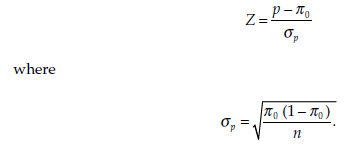
It follows a standard normal distribution.

Interpreting the test The decision rules are the following:

• in a two-tail test, H₀ will be rejected if Z <- Z_a/2 or Z > Z_a/2
• in a left-tail test, H₀ will be rejected if Z < – Z_a
• in a right-tail test, H₀ will be rejected if Z > Z_a.

2.2. Comparing two proportions or percentages p₁ and p₂ (with large samples)

Research question Do the two proportions or percentages p₁ and p₂, observed in two samples, differ significantly?

Application conditions

• The two samples are random and contain n₁ and n₂ independent observa­tions respectively.
• The distribution of the proportion in each population is binomial.
• Both samples are large (n₁ > 30 and n₂ > 30).

Hypotheses

Null hypothesis, H₀: π₁ = π₂,

alternative hypothesis, H1: π₁ # π₂ (for a two-tail test)

or H1: π₁ < π₂ (for a left-tail test)

or H1: π₁ > π₂ (for a right-tail test).

Statistic

The statistic calculated is

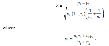
It follows a standard normal distribution.

Interpreting the test The decision rules are the following:

• in a two-tail test, H₀ will be rejected if Z <- Z_a/2 or Z > Z_a/2
• in a left-tail test, H₀ will be rejected if Z <- Z_a
• in a right-tail test, H₀ will be rejected if Z > Z_a.

2.3. Comparing k proportions or percentages p_k (large samples)

Research question Do the k proportions or percentages p₁, p₂… , p_k, observed in k samples, differ significantly from each other?

Application conditions

• The k samples are random and contain n1 n₂… n_k independent observations.
• The distribution of the proportion or percentage is binomial in each of the k
• All the samples are large (n₁, n₂… and n_k > 50).
• The k proportions p_k as well as their complements 1 – p_k represent at least five observations, that is: p_kxn_k > 5 and (1 – p_k) xn_k > 5

Hypotheses

Null hypothesis, H₀: π₁ = π₂ = … = π_k,

alternative hypothesis, H₁: the values of π_i (i = 1, 2, … , k) are not all identical. This means that one single different value would be enough to reject the null hypothesis, thus validating the alternative hypothesis.

Statistic

The statistic calculated is

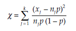
where xj = the number of observations in the sample j corresponding to the pro­portion pj, and

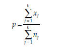
The statistic % follows a chi-square distribution, with k – 1 degrees of freedom.

Interpreting the test The decision rule is the following:

H₀ will be rejected if

3. Variance Test

3.1. Comparing the variance σ² to a reference value σ²0

Research question Does the variance s² calculated from a sample differ signifi­cantly from a hypothetical variance σ²0 ?

Application conditions

• The sample is random and contains n independent observations.
• The distribution of the variance in the population is normal, the mean and standard deviation are not known.

Hypotheses

Null hypothesis, H₀: σ² = σ²₀,

alternative hypothesis, H1 σ² # σ²₀ (for a two-tail test)

or H1 σ² < σ²₀ (for a left-tail test)

or H1 σ² > σ²₀ (for a right-tail test).

Statistic

The statistic calculated is

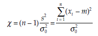
where σ²₀ is the given variance, s² the variance estimated from the sample, and m the mean estimated from the sample. The statistic % follows a chi-square dis­tribution with n – 1 degrees of freedom, which is written x²(n – 1).

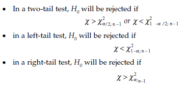
Interpreting the test The decision rules are the following:

3.2. Comparing two variances

Research question Do the variances o0 and o2 of two populations differ significantly from each other?

Application conditions

• Both samples are random and contain n₁ and n₂ independent observations respectively.
• The distribution of the variance of each population is normal, or the samples are large (n₁ > 30 and n₂ > 30).

Hypotheses

Null hypothesis, H₀: σ²₁ = σ²₂,

alternative hypothesis, H1 σ²₁ # σ²₂ (for a two-tail test)

or H1 σ²₁ < σ²₂ (for a left-tail test)

or H1 σ²₁ > σ²₂ (for a right-tail test).

Statistic

The statistic calculated is

Where

and

x_1i = the value of variable X for observation i in population 1,

x_2i = the value of variable X for observation i in population 2,

x₁ = the mean estimated from the sample of variable X in population 1,

x₂ = the mean estimated from the sample of variable X in population 2.

If required, the numbering of the samples may be inverted to give the numerator the greater of the two estimated variances,

The statistic F follows a Fisher-Snedecor distribution, F(n₁ – 1, n₂ – 1). Interpreting the test The decision rules are the following:

• ^{In a two-tail tes}b H0 ^wib ^{be re}j^{ected if F} > ^F_a/₂. n1 _ 1, n2 – 1 ^{or F} < ^F1 – a/2; n1 – 1, n2 – 1
• in a left-tail test, H₀ will be rejected if F > F_a. _n2 _ ₁, _n1 _ ₁
• in a right-tail test, H₀ will be rejected if F > F_a. _n1 _ ₁, _n2 _ ₁.

3.3. Comparing k variances: Bartlett test

Research question Do k variances σ²_{1 ,} σ²_{2 ,} ….σ²_k observed in k samples, differ significantly from each other?

Application conditions

• All k samples are random and contain n₁, n₂… n_k independent observations.
• The distribution of the variance of all k populations is normal.
• None of the observed variances equals zero.

Hypotheses

Null hypothesis, H₀:

alternative hypothesis, H₁: the values of of (i = 1, 2, … , k) are not identical

Statistic

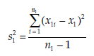
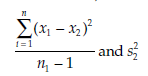
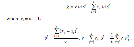
The statistic calculated is

Xj = the value of variable X for observation j in population i,

x_i = the mean of variable X in population i, estimated from a sample of size n_i,

s2 = the variance of variable X in population i, estimated from a sample of size n.

The statistic % follows a chi-square distribution with v degrees of freedom.

Interpreting the test The decision rule is the following:

H₀ will be rejected if

3.4. Comparing k variances: Cochran test

Research question Do k variances σ²_{1 ,} σ²_{2 ,} ….σ²_k observed in k samples, differ significantly from each other?

More precisely, the Cochran test examines if the greatest of the k variances is significantly different to the k – 1 other variances

Application conditions

• The k samples are random and contain a same number n of independent observations.
• The variance in each of the k populations follows a normal distribution, or at least a uni-modal distribution.

Hypotheses

Null hypothesis, H₀: σ²₁ =σ²_{2 ,} =…σ²_k

alternative hypothesis, H₁: the values of σ²_i (i = 1, 2, … , k) are not identical.

Statistic

The statistic calculated is

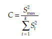
where the values of s2i 2 are the estimated variances calculated with n = n – 1 degrees of freedom, and S2 max is the greatest estimated variance within the k samples.

The statistic C is compared to the critical value Ca, as read from a table.

Interpreting the test The decision rule is the following: H₀ will be rejected if C > C_a.

4. Correlation Tests

4.1. Comparing a linear correlation coefficient r to zero

Research question Is the linear correlation coefficient r of two variables X and Y significant – that is, not equal to zero?

Application conditions

• The observed variables X and Y are, at least, continuous variables.

Hypotheses

Null hypothesis, H₀: p = 0,

alternative hypothesis, H₁: p # 0 (for a two-tail test)

or H₁: p < 0 (for a left-tail test)

or H₁: p > 0 (for a right-tail test)

Statistic

The statistic calculated is

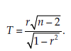
It follows a Student distribution with n – 2 degrees of freedom.

Interpreting the test The decision rules are the following:

• in a two-tail test, H₀ will be rejected if T <- T_{a/2; n} _ ₂ or T > T_{a/2; n} _ ₂
• in a left-tail test, H₀ will be rejected if T <- T_a. _n _ ₂
• in a right-tail test, H₀ will be rejected if T > T_a. _n _ ₂.

For large values of n (n – 2 > 30), this statistic approximates a standard nor­mal distribution. The decision to reject or not to reject the null hypothesis can then be made by comparing the calculated statistic T to values of the standard normal distribution, using the decision rules that have already been presented earlier in this chapter.

4.2. Comparing a linear correlation coefficient r to a reference value p₀

Research question Is the linear correlation coefficient r of two variables X and Y, calculated from a sample, significantly different from a hypothetical refer­ence value r ₀?

Application conditions

• The observed variables X and Y are, at least, continuous variables.

Hypotheses

Null hypothesis, H₀: p = p₀,

alternative hypothesis, H1. p # p₀ (for a two-tail test)

or Hy. p < p₀ (for a left-tail test)

or Hy p > p₀ (for a right-tail test)

Statistic

The statistic calculated is

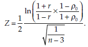
It follows a standard normal distribution.

Interpreting the test The decision rules are the following:

• in a two-tail test, H₀ will be rejected if Z <- Z_a/2 or Z > Z_a/2
• in a left-tail test, H₀ will be rejected if Z <- Z_a
• in a right-tail test, H₀ will be rejected if Z > Z_a.

4.3. Comparing two linear correlation coefficients, p ₁ and p₂

Research question Do the two linear correlation coefficients p ₁ and p₂ differ significantly from each other?

Application conditions

• The two linear correlation coefficients r₁ and r₂ are obtained from two samples of size n₁ and n₂ respectively.

Hypotheses

Null hypothesis, H₀: p ₁ = p ₂,

alternative hypothesis, Hy p ₁ # p₂ (for a two-tail test)

or Hy p ₁ < p₂ (for a left-tail test)

or Hy p ₁ > p₂ (for a right-tail test).

Statistic

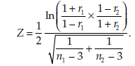
The statistic calculated is

It follows a standard normal distribution.

Interpreting the test The decision rules are thus the following:

• in a two-tail test, H₀ will be rejected if Z <- Z_{a/2 or} Z > Z_a/2
• in a left-tail test, H₀ will be rejected if Z <- Z_a
• in a right-tail test, H₀ will be rejected if Z > Z_a.

5. Regression Coefficient Tests

5.1. Comparing a linear regression coefficient b to zero

Research question Is the linear regression coefficient P of two variables X and Y significant, that is, not equal to zero?

Application conditions

• The observed variables X and Y are, at least, continuous variables.
• P follows a normal distribution or the size n of the sample is greater than 30.

Hypotheses

Null hypothesis, H₀: P = 0,

alternative hypothesis, H₁: P # 0 (for a two-tail test)

or H₁: P < 0 (for a left-tail test)

or H₁: P > 0 (for a right-tail test).

Statistic

The statistic calculated is

where b represents the regression coefficient P and s_h its standard deviation, both estimated from the sample. The statistic T follows a Student distribution with n – 2 degrees of freedom.

Interpreting the test The decision rules are the following:

• in a two-tail test, H₀ will be rejected if T <- T_{a/2; n} _ ₂ or T > T_{a/2; n} _ ₂
• in a left-tail test, H₀ will be rejected if T <- T_a. _n _ ₂
• in a right-tail test, H₀ will be rejected if T > T_a. _n _ ₂.

5.2. Comparing a linear regression coefficient β to a reference value β₀

Research question Is the linear regression coefficient b of two variables X and Y significantly different from a reference value β₀?

Application conditions

• The observed variables X and Y are, at least, continuous variables.
• P follows a normal distribution or the size n of the sample is greater than 30.

Hypotheses

Null hypothesis, H₀: β = β₀,

alternative hypothesis, Hp β # β₀ (for a two-tail test)

or Hp β < β₀ (for a left-tail test)

or Hp β > β₀ (for a right-tail test).

Statistic

The statistic calculated is

where b represents the regression coefficient P and s_ its standard deviation, both estimated from the sample. The statistic T follows a Student distribution with n – 2 degrees of freedom.

Interpreting the test The decision rules are the following:

• in a two-tail test, H₀ will be rejected if T <- T_{a/2; n} _ ₂ or T > T_{a/2; n} _ ₂
• in a left-tail test, H₀ will be rejected if T <- T_a. _n _ ₂
• in a right-tail test, H₀ will be rejected if T > T_a. _n _ ₂.

5.3. Comparing two linear regression coefficients β and β in two populations

Research question Do the two linear regression coefficients β and β’, observed in two populations, differ significantly from each other?

This is again a situation in which the difference between two means b and _ with estimated variances s2b, and s2b, is tested. Naturally we must distinguish between cases in which the two variances are equal and cases in which they are not equal. If these variances differ, an Aspin-Welch test will be used.

Application conditions

• β and β’ represent the values of the regression coefficient in two popula­tions, from which two independent, random samples have been selected.
• The observed variables X and Y are, at least, continuous variables.

Hypotheses

Null hypothesis, H₀: β = β’,

alternative hypothesis, H₁ : β # β’ (for a two-tail test)

or H₁ : β < β’ (for a left-tail test)

or H₁ : β > β’  (for a right-tail test).

Statistic

The statistics calculated and the interpretations of the tests are the same as for the tests on differences of means, described in parts 1.1 through 1.5 in this chapter.

In addition, it is possible to use the same kind of tests on a constant (P ₀) of the linear regression equation. However, this practice is rarely used due to the great difficulties in interpreting the results. Similarly, more than two regression coefficients may be compared. For instance, the Chow test (Chow, 1960; Toyoda, 1974), which uses the Fisher-Snedecor distribution, is used to determine whether the coefficients of a regression equation are the same in two or more groups. This is called an omnibus test, which means that it tests whether the full set of equation coefficients are identical.

When comparing two groups, a neat and quite simple alternative to the Chow test is the introduction of a ‘dummy variable’ to the regression, indicat­ing the group it belongs to. The original variables are multiplied by the dummy variable thus obtaining a set of new variables. The coefficients of the dummy variable represent the differences between the constants (P ₀) for the two groups, and the coefficients of the new variables represent the differences between the coefficients of the explicative variables for the two groups. These coefficients can then be tested globally (as the Chow test does) or individually (see Sections 5.1 through 5.3 in this chapter) to identify which coefficient behaves differently according to the group.

Source: Thietart Raymond-Alain et al. (2001), Doing Management Research: A Comprehensive Guide, SAGE Publications Ltd; 1 edition.