Time Series Decomposition

In this section we turn our attention to what is called time series decomposition. Time series decomposition can be used to separate or decompose a time series into seasonal, trend, and irregular components. While this method can be used for forecasting, its primary applicability is to get a better understanding of the time series. Many business and economic time series are maintained and published by government agencies such as the Census Bureau and the Bureau of Labor Statistics. These agencies use time series decom­position to create deseasonalized time series.

Understanding what is really going on with a time series often depends upon the use of deseasonalized data. For instance, we might be interested in learning whether electrical power consumption is increasing in our area. Suppose we learn that electric power consumption in September is down 3% from the previous month. Care must be exercised in using such information, because whenever a seasonal influence is present, such comparisons may be misleading if the data have not been deseasonalized. The fact that electric power consumption is down 3% from August to September might be only the seasonal effect associated with a decrease in the use of air conditioning and not because of a long-term decline in the use of electric power. Indeed, after adjusting for the seasonal effect, we might even find that the use of electric power increased. Many other time series, such as unemployment statistics, home sales, and retail sales, are subject to strong seasonal influences. It is important to deseasonalize such data before making a judgment about any long-term trend.

Time series decomposition methods assume that Y,, the actual time series value at period t, is a function of three components: a trend component; a seasonal component; and an irregular or error component. How these three components are combined to generate the observed values of the time series depends upon whether we assume the relationship is best described by an additive or a multiplicative model.

An additive decomposition model takes the following form:

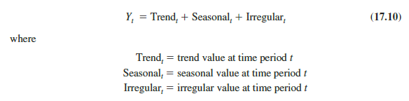
In an additive model the values for the three components are simply added together to obtain the actual time series value Y,. The irregular or error component accounts for the variability in the time series that cannot be explained by the trend and seasonal components.

An additive model is appropriate in situations where the seasonal fluctuations do not depend upon the level of the time series. The regression model for incorporating seasonal and trend effects in Section 17.5 is an additive model. If the sizes of the seasonal fluctu­ations in earlier time periods are about the same as the sizes of the seasonal fluctuations in later time periods, an additive model is appropriate. However, if the seasonal fluctuations change over time, growing larger as the sales volume increases because of a long-term linear trend, then a multiplicative model should be used. Many business and economic time series follow this pattern.

A multiplicative decomposition model takes the following form:

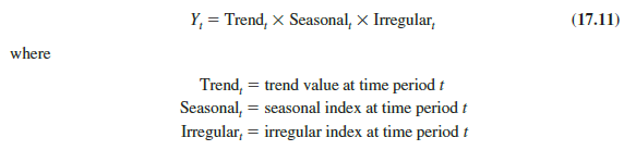
In this model, the trend and seasonal and irregular components are multiplied to give the value of the time series. Trend is measured in units of the item being forecast. How­ever, the seasonal and irregular components are measured in relative terms, with values above 1.00 indicating effects above the trend and values below 1.00 indicating effects below the trend.

Because this is the method most often used in practice, we will restrict our discus­sion of time series decomposition to showing how to develop estimates of the trend and seasonal components for a multiplicative model. As an illustration, we will work with the quarterly smartphone sales time series introduced in Section 17.5; the quarterly sales data are shown in Table 17.18 and the corresponding time series plot is presented in Fig­ure 17.18. After demonstrating how to decompose a time series using the multiplicative model, we will show how the seasonal indices and trend component can be recombined to develop a forecast.

1. Calculating the Seasonal Indexes

Figure 17.18 indicates that sales are lowest in the second quarter of each year and increase in quarters 3 and 4. Thus, we conclude that a seasonal pattern exists for the smartphone sales time series. The computational procedure used to identify each quarter’s seasonal influence begins by computing a moving average to remove the combined seasonal and irregular ef­fects from the data, leaving us with a time series that contains only trend and any remaining random variation not removed by the moving average calculations.

Because we are working with a quarterly series, we will use four data values in each moving average. The moving average calculation for the first four quarters of the smartphone sales data is

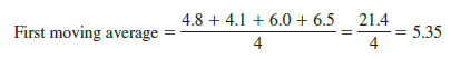
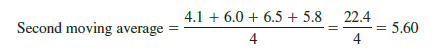
Note that the moving average calculation for the first four quarters yields the average quar­terly sales over year 1 of the time series. Continuing the moving average calculations, we next add the 5.8 value for the first quarter of year 2 and drop the 4.8 for the first quarter of year 1. Thus, the second moving average is

Similarly, the third moving average calculation is (6.0 + 6.5 + 5.8 + 5.2)/4 = 5.875.

Before we proceed with the moving average calculations for the entire time series, let us return to the first moving average calculation, which resulted in a value of 5.35. The 5.35 value is the average quarterly sales volume for year 1. As we look back at the calculation of the 5.35 value, associating 5.35 with the “middle” of the moving average group makes sense. Note, however, that with four quarters in the moving average, there is no middle period.

The 5.35 value really corresponds to period 2.5, the last half of quarter 2 and the first half of quarter 3. Similarly, if we go to the next moving average value of 5.60, the middle period corresponds to period 3.5, the last half of quarter 3 and the first half of quarter 4.

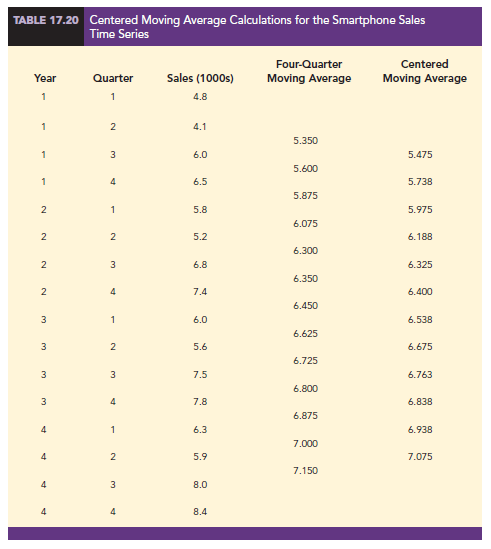
The two moving average values we computed do not correspond directly to the original quarters of the time series. We can resolve this difficulty by computing the average of the two moving averages. Since the center of the first moving average is period 2.5 (half a period or quarter early) and the center of the second moving average is period 3.5 (half a period or quarter late), the average of the two moving averages is centered at quarter 3, exactly where it should be. This moving average is referred to as a centered moving average. Thus, the centered moving average for period 3 is (5.35 + 5.60)/2 = 5.475. Similarly, the centered moving average value for period 4 is (5.60 + 5.875)/2 = 5.738. Table 17.20 shows a complete summary of the moving average and centered moving average calculations for the smartphone sales data.

What do the centered moving averages in Table 17.20 tell us about this time series? Figure 17.20 shows a time series plot of the actual time series values and the centered moving average values. Note particularly how the centered moving average values tend to “smooth out” both the seasonal and irregular fluctuations in the time series. The centered moving averages represent the trend in the data and any random variation that was not removed by using moving averages to smooth the data.

Previously we showed that the multiplicative decomposition model is

Y_t = Trend_t X Seasonal_t X Irregular_t

By dividing each side of this equation by the trend component Trendt , we can identify the combined seasonal-irregular effect in the time series.

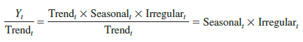
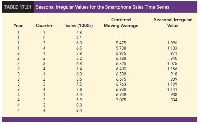
For example, the third quarter of year 1 shows a trend value of 5.475 (the centered mov­ing average). So 6.0/5.475 = 1.096 is the combined seasonal-irregular value. Table 17.21 summarizes the seasonal-irregular values for the entire time series.

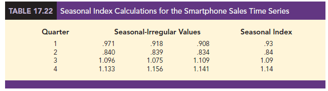
Consider the seasonal-irregular values for the third quarter: 1.096, 1.075, and 1.109. Seasonal-irregular values greater than 1.00 indicate effects above the trend estimate and values below 1.00 indicate effects below the trend estimate. Thus, the three seasonal-irregular values for quarter 3 show an above-average effect in the third quarter. Since the year-to- year fluctuations in the seasonal-irregular values are primarily due to random error, we can average the computed values to eliminate the irregular influence and obtain an estimate of the third-quarter seasonal influence.

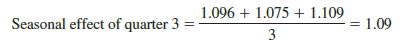
We refer to 1.09 as the seasonal index for the third quarter. Table 17.22 summarizes the calculations involved in computing the seasonal indexes for the smartphone sales time series. The seasonal indexes for the four quarters are .93, .84, 1.09, and 1.14.

Interpretation of the seasonal indexes in Table 17.22 provides some insight about the seasonal component in smartphone sales. The best sales quarter is the fourth quarter, with sales averaging 14% above the trend estimate. The worst, or slowest, sales quarter is the second quarter; its seasonal index of .84 shows that the sales average is 16% below the trend estimate. The seasonal component corresponds to the intuitive expectation that cell phone sales increase when a new school year begins in quarter three and and for the holiday season (quarter four).

One final adjustment is sometimes necessary in obtaining the seasonal indexes. Because the multiplicative model requires that the average seasonal index equals 1.00, the sum of the four seasonal indexes in Table 17.22 must equal 4.00. In other words, the seasonal effects must even out over the year. The average of the seasonal indexes in our example is equal to 1.00, and hence this type of adjustment is not necessary. In other cases, a slight adjustment may be necessary. To make the adjustment, multiply each seasonal index by the number of seasons di­vided by the sum of the unadjusted seasonal indexes. For instance, for quarterly data, multiply each seasonal index by 4/(sum of the unadjusted seasonal indexes). Some of the exercises will require this adjustment to obtain the appropriate seasonal indexes.

2. Deseasonalizing the Time Series

A time series that has had the seasonal effects removed is referred to as a deseasonalized time series, and the process of using the seasonal indexes to remove the seasonal effects from a time series is referred to as deseasonalizing the time series. Using a multiplicative decomposition model, we deseasonalize a time series by dividing each observation by its corresponding seasonal index. The multiplicative decomposition model is

Y_t = Trend_t X Seasonal, X Irregular_t

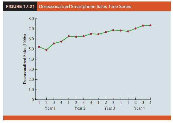
So, when we divide each time series observation (Y_t) by its corresponding seasonal index, the resulting data show only trend and random variability (the irregular component). The deseasonalized time series for smartphone sales is summarized in Table 17.23. A graph of the deseasonalized time series is shown in Figure 17.21.

3. Using the Deseasonalized Time Series to Identify Trend

The graph of the deseasonalized smartphone sales time series shown in Figure 17.21 appears to have an upward linear trend. To identify this trend, we will fit a linear trend equation to the deseasonalized time series using the same method shown in Section 17.4. The only difference is that we will be fitting a trend line to the deseasonalized data instead of the original data.

Recall that for a linear trend the estimated regression equation can be written as

^Tt = ^b0 + ^b1^t

where

T_t = linear trend forecast in period t

b₀ = intercept of the linear trend line

b₁ = slope of the trend line

t = time period

In Section 17.4 we provided formulas for computing the values of b₀ and b₁. To fit a linear trend line to the deseasonalized data in Table 17.23, the only change is that the deseasonal­ized time series values are used instead of the observed values Y_t in computing b₀ and b₁.

Figure 17.22 shows a portion of the computer output obtained using regression analysis to estimate the trend line for the deseasonalized smartphone time series. The estimated linear trend equation is

Deseasonalized Sales = 5.104 + .1476t

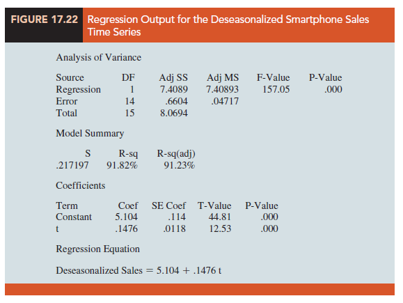
The slope of .1476 indicates that over the past 16 quarters, the firm averaged a de­seasonalized growth in sales of about 148 sets per quarter. If we assume that the past 16-quarter trend in sales data is a reasonably good indicator of the future, this equation can be used to develop a trend projection for future quarters. For example, substituting t = 17 into the equation yields next quarter’s deseasonalized trend projection, T₁₇.

T₁₇ = 5.104 + .1476(17) = 7.613

Thus, using the deseasonalized data, the linear trend forecast for next quarter (period 17) is 7613 smartphones. Similarly, the deseasonalized trend forecasts for the next three quarters (periods 18, 19, and 20) are 7761, 7908, and 8056 smartphones, respectively.

4. Seasonal Adjustments

The final step in developing the forecast when both trend and seasonal components are present is to use the seasonal indexes to adjust the deseasonalized trend projections.

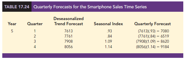
Returning to the smartphone sales example, we have a deseasonalized trend projection for the next four quarters. Now we must adjust the forecast for the seasonal effect. The seasonal index for the first quarter of year 5 (t = 17) is .93, so we obtain the quarterly forecast by mul­tiplying the deseasonalized forecast based on trend (T₁₇ = 7616) by the seasonal index (.93). Thus, the forecast for the next quarter is 7616(.93) = 7083. Table 17.24 shows the quarterly forecast for quarters 17 through 20. The high-volume fourth quarter has a 9188-unit forecast, and the low-volume second quarter has a 6522-unit forecast.

5. Models Based on Monthly Data

In the preceding smartphone sales example, we used quarterly data to illustrate the com­putation of seasonal indexes. However, many businesses use monthly rather than quarterly forecasts. In such cases, the procedures introduced in this section can be applied with minor modifications. First, a 12-month moving average replaces the four-quarter moving average; second, 12 monthly seasonal indexes, rather than four quarterly seasonal indexes, must be computed. Other than these changes, the computational and forecasting procedures are identical.

6. Cyclical Component

Mathematically, the multiplicative model of equation (17.11) can be expanded to include a cyclical component.

The cyclical component, like the seasonal component, is expressed as a percentage of trend. As mentioned in Section 17.1, this component is attributable to multiyear cycles in the time series. It is analogous to the seasonal component, but over a longer period of time. However, because of the length of time involved, obtaining enough relevant data to estimate the cyclical component is often difficult. Another difficulty is that cycles usually vary in length. Because it is so difficult to identify and/or separate cyclical effects from long-term trend effects, in practice these effects are often combined and referred to as a combined trend-cycle component. We leave further discussion of the cyclical component to specialized texts on forecasting methods.

Source:  Anderson David R., Sweeney Dennis J., Williams Thomas A. (2019), Statistics for Business & Economics, Cengage Learning; 14th edition.