In this section we show how to develop forecasts for a time series that has a seasonal pattern. To the extent that seasonality exists, we need to incorporate it into our forecasting models to ensure accurate forecasts. We begin by considering a seasonal time series with no trend and then discuss how to model seasonality with trend.
1. Seasonality Without Trend
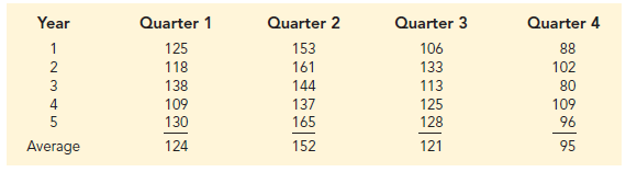
As an example, consider the number of umbrellas sold at a clothing store over the past five years. Table 17.16 shows the time series and Figure 17.16 shows the corresponding time series plot. The time series plot does not indicate any long-term trend in sales. In fact, unless you look carefully at the data, you might conclude that the data follow a horizontal pattern and that single exponential smoothing could be used to forecast sales. But closer inspection of the time series plot reveals a pattern in the data. That is, the first and third quarters have moderate sales, the second quarter has the highest sales, and the fourth quarter tends to be the lowest quarter in terms of sales volume. Thus, we would conclude that a quarterly seasonal pattern is present.
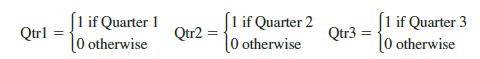
Just like using dummy variables to deal with an independent variable in a standard regression analysis, we can use the same approach to model a time series with a seasonal pattern by treating the season as a categorical variable. Recall that when a categorical variable has k levels, k – 1 dummy variables are required. So, if there are four seasons, we need three dummy variables. For instance, in the umbrella sales time series season is a categorical variable with four levels: quarter 1, quarter 2, quarter 3, and quarter 4. Thus, to model the seasonal effects in the umbrella time series we need 4 – 1=3 dummy variables. The three dummy variables can be coded as follows:
Using Yˆ to denote the estimated or forecasted value of sales, the general form of the estimated regression equation relating the number of umbrellas sold to the quarter the sales take place follows:
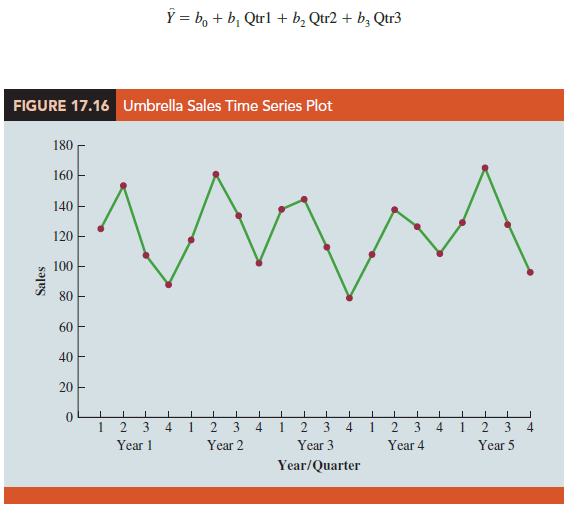
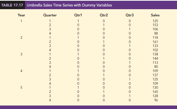
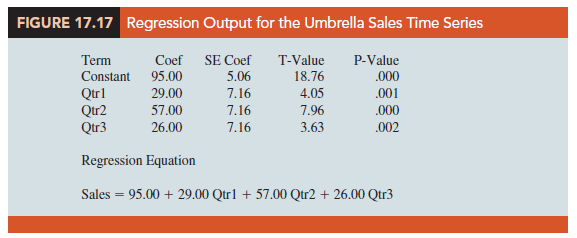
Table 17.17 is the umbrella sales time series with the coded values of the dummy variables shown. Using the data in Table 17.17, we obtained the computer output, a portion of which is shown in Figure 17.17. The estimated multiple regression equation obtained is
Sales = 95.00 + 29.00 Qtr1 + 57.00 Qtr2 + 26.00 Qtr3
We can use this equation to forecast quarterly sales for next year.
Quarter 1: Sales = 95.0 + 29.0(1) + 57.0(0) + 26.0(0) = 124
Quarter 2: Sales = 95.0 + 29.0(0) + 57.0(1) + 26.0(0) = 152
Quarter 3: Sales = 95.0 + 29.0(0) + 57.0(0) + 26.0(1) = 121
Quarter 4: Sales = 95.0 + 29.0(0) + 57.0(1) + 26.0(0) = 95
It is interesting to note that we could have obtained the quarterly forecasts for next year simply by computing the average number of umbrellas sold in each quarter, as shown in the following table.
Nonetheless, the regression output shown in Figure 17.17 provides additional information that can be used to assess the accuracy of the forecast and determine the significance of the results. And, for more complex types of problem situations, such as dealing with a time series that has both trend and seasonal effects, this simple averaging approach will not work.
2. Seasonality and Trend
Let us now extend the regression approach to include situations where the time series contains both a seasonal effect and a linear trend by showing how to forecast the quarterly smartphone sales time series introduced in Section 17.1. The data for the smartphone time series are shown in Table 17.18. The time series plot in Figure 17.18 indicates that sales are lowest in the second quarter of each year and increase in quarters 3 and 4. Thus, we conclude that a seasonal pattern exists for smartphone sales. But the time series also has an upward linear trend that will need to be accounted for in order to develop accurate forecasts of quarterly sales. This is easily handled by combining the dummy variable approach for seasonality with the time series regression approach we discussed in Section 17.3 for handling linear trend.

The general form of the estimated multiple regression equation for modeling both the quarterly seasonal effects and the linear trend in the smartphone time series is as follows:
![]()
where
Yt = estimate or forecast of sales in period t
Qtrl = 1 if time period t corresponds to the first quarter of the year; 0 otherwise
Qtr2 = 1 if time period t corresponds to the second quarter of the year; 0 otherwise
Qtr3 = 1 if time period t corresponds to the third quarter of the year; 0 otherwise t = time period
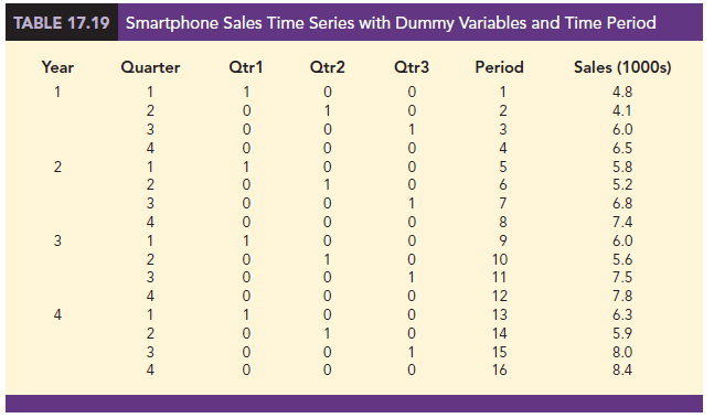
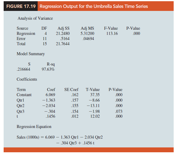
Table 17.19 is the revised smartphone sales time series that includes the coded values of the dummy variables and the time period t. Using the data in Table 17.19, we obtained the computer output shown in Figure 17.19. The estimated multiple regression equation is
Sales (1000s) = 6.069 – 1.363 Qtr1 – 2.034 Qtr2 – .304 Qtr3 + .1456t (17.9)
We can now use equation (17.9) to forecast quarterly sales for next year. Next year is year 5 for the smartphone sales time series; that is, time periods 17, 18, 19, and 20.
Forecast for Time Period 17 (Quarter 1 in Year 5)
Sales (1000s) = 6.069 – 1.363(1) – 2.034(0) – .304(0) + .1456(17) = 7.18
Forecast for Time Period 18 (Quarter 2 in Year 5)
Sales (1000s) = 6.069 – 1.363(0) – 2.034(1) – .304(0) + .1456(18) = 6.66
Forecast for Time Period 19 (Quarter 3 in Year 5)
Sales = 6.069 – 1.363(0) – 2.034(0) – .304(1) + .1456(19) = 8.53
Forecast for Time Period 20 (Quarter 4 in Year 5)
Sales = 6.069 – 1.363(0) – 2.034(0) – .304(0) + .1456(20) = 8.98
Thus, accounting for the seasonal effects and the linear trend in smartphone sales, the estimates of quarterly sales in year 5 are 7180, 6660, 8530, and 8980.
The dummy variables in the estimated multiple regression equation actually provide four estimated multiple regression equations, one for each quarter. For instance, if time period t corresponds to quarter 1, the estimate of quarterly sales is
Quarter 1: Sales = 6.069 – 1.363(1) – 2.034(0) – .304(0) + .1456(t) = 4.71 + .1456t
Similarly, if time period t corresponds to quarters 2, 3, and 4, the estimates of quarterly sales are
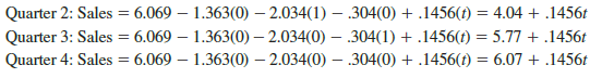
The slope of the trend line for each quarterly forecast equation is .1456, indicating a growth in sales of about 146 sets per quarter. The only difference in the four equations is that they have different intercepts. For instance, the intercept for the quarter 1 equation is 4.71 and the intercept for the quarter 4 equation is 6.07. Thus, sales in quarter 1 are 4.71 – 6.07 = -1.36 or 1360 sets less than in quarter 4. In other words, the estimated regression coefficient for Qtr1 in equation (17.9) provides an estimate of the difference in sales between quarter 1 and quarter 4. Similar interpretations can be provided for −2.03, the estimated regression coefficient for dummy variable Qtr2, and −.304, the estimated regression coefficient for dummy variable Qtr3.
3. Models Based on Monthly Data
In the preceding smartphone sales example, we showed how dummy variables can be used to account for the quarterly seasonal effects in the time series. Because there were 4 levels for the categorical variable season, 3 dummy variables were required. However, many businesses use monthly rather than quarterly forecasts. For monthly data, season is a categorical variable with 12 levels and thus 12 – 1 = 11 dummy variables are required. For example, the 11 dummy variables could be coded as follows:
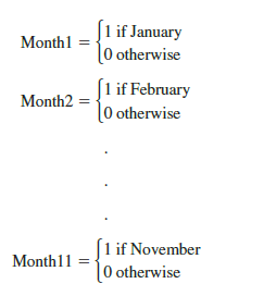
Other than this change, the multiple regression approach for handling seasonality remains the same.
Source: Anderson David R., Sweeney Dennis J., Williams Thomas A. (2019), Statistics for Business & Economics, Cengage Learning; 14th edition.
I believe you have remarked some very interesting points, regards for the post.