The sign test is a versatile nonparametric method for hypothesis testing that uses the binomial distribution with p = .50 as the sampling distribution. It does not require an assumption about the distribution of the population. In this section we present two applications of the sign test: one involving a hypothesis test about a population median and one involving a matched-sample test about the difference between two populations.
1. Hypothesis Test About a Population Median
In this section, we show how the sign test can be used to conduct a hypothesis test about a population median. If we consider a population where no data value is exactly equal to the median, the median is the measure of central tendency that divides the population so that 50% of the values are greater than the median and 50% of the values are less than the median. Whenever a population distribution is skewed, the median is often preferred over the mean as the best measure of central location for the population. The sign test provides a nonparametric procedure for testing a hypothesis about the value of a population median.
In order to demonstrate the sign test, we consider the weekly sales of Cape May Potato Chips by the Lawler Grocery Store chain. Lawler’s management made the decision to carry the new potato chip product based on the manufacturer’s estimate that the median sales should be $450 per week on a per store basis. After carrying the product for three- months, Lawler’s management requested the following hypothesis test about the population median weekly sales:
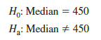
Data showing one-week sales at 10 randomly selected Lawler’s stores are provided in Table 18.1.
In conducting the sign test, we compare each sample observation to the hypothesized value of the population median. If the observation is greater than the hypothesized value, we record a plus sign “ + .” If the observation is less than the hypothesized value, we record a minus sign “—.” If an observation is exactly equal to the hypothesized value, the observation is eliminated from the sample and the analysis proceeds with the smaller sample size, using only the observations where a plus sign or a minus sign has been recorded. It is the conversion of the sample data to either a plus sign or a minus sign that gives the nonparametric method its name: the sign test.

Consider the sample data in Table 18.1. The first observation, 485, is greater than the hypothesized median 450; a plus sign is recorded. The second observation, 562, is greater than the hypothesized median 450; a plus sign is recorded. Continuing with the 10 observations in the sample provides the plus and minus signs as shown in Table 18.2. Note that there are 7 plus signs and 3 minus signs.
The assigning of the plus signs and minus signs has made the situation a binomial distribution application. The sample size n = 10 is the number of trials. There are two outcomes possible per trial, a plus sign or a minus sign, and the trials are independent. Let p denote the probability of a plus sign. If the population median is 450, p would equal .50 as there should be 50% plus signs and 50% minus signs in the population. Thus, in terms of the binomial probability p, the sign test hypotheses about the population median
are converted to the following hypotheses about the binomial probability p.

If H0 cannot be rejected, we cannot conclude that p is different from .50 and thus we cannot conclude that the population median is different from 450. However, if H0 is rejected, we can conclude that p is not equal to .50 and thus the population median is not equal to 450.
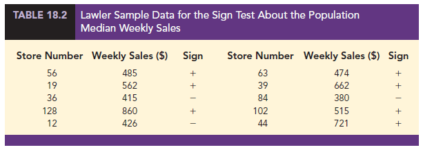
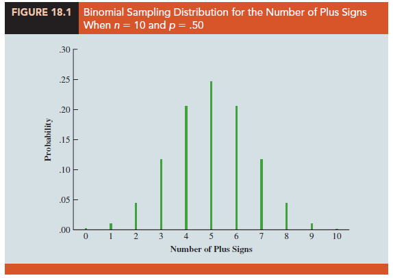
With n = 10 stores or trials and p = .50, we used Table 5 in Appendix B to obtain the binomial probabilities for the number of plus signs under the assumption H0 is true. These probabilities are shown in Table 18.3. Figure 18.1 shows a graphical representation of this binomial distribution.
Let us proceed to show how the binomial distribution can be used to test the hypothesis about the population median. We will use a .10 level of significance for the test. Since the observed number of plus signs for the sample data, 7, is in the upper tail of the binomial distribution, we begin by computing the probability of obtaining 7 or more plus signs. This probability is the probability of 7, 8, 9, or 10 plus signs. Adding these probabilities shown in Table 18.3, we have .1172 + .0439 + .0098 + .0010 = .1719. Since we are using a two-tailed hypothesis test, this upper tail probability is doubled to obtain the p-value = 2(.1719) = .3438. With p-value > a, we cannot reject H0. In terms of the binomial probability p, we cannot reject H0: p = .50, and thus we cannot reject the hypothesis that the population median is $450.
In this example, the hypothesis test about the population median was formulated as a two-tailed test. However, one-tailed sign tests about a population median are also possible. For example, we could have formulated the hypotheses as an upper tail test so that the null and alternative hypotheses would be written as follows:
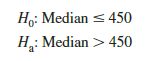
The corresponding p-value is equal to the binomial probability that the number of plus signs is greater than or equal to 7 found in the sample. This one-tailed p-value would have been .1172 + .0439 + .0098 + .0010 = .1719. If the example were converted to a lower tail test, the p-value would have been the probability of obtaining 7 or fewer plus signs.
The application we have just described makes use of the binomial distribution with p = .50. The binomial probabilities provided in Table 5 of Appendix B can be used to compute the p-value when the sample size is 20 or less. With larger sample sizes, we rely on the normal distribution approximation of the binomial distribution to compute the p-value; this makes the computations quicker and easier. A large sample application of the sign test is illustrated in the following example.
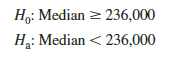
One year ago the median price of a new home was $236,000. However, a current downturn in the economy has real estate firms using sample data on recent home sales to determine if the population median price of a new home is less today than it was a year ago. The hypothesis test about the population median price of a new home is as follows:
We will use a .05 level of significance to conduct this test.
A random sample of 61 recent new home sales found 22 homes sold for more than $236,000, 38 homes sold for less than $236,000, and one home sold for $236,000. After deleting the home that sold for the hypothesized median price of $236,000, the sign test continues with 22 plus signs, 38 minus signs, and a sample of 60 homes.
The null hypothesis that the population median is greater than or equal to $236,000 is expressed by the binomial distribution hypothesis H0: p > .50. If H0 were true as an equality, we would expect .50(60) = 30 homes to have a plus sign. The sample result showing 22 plus signs is in the lower tail of the binomial distribution. Thus, the p-value is the probability of 22 or fewer plus signs when p = .50. While it is possible to compute the exact binomial probabilities for 0, 1, 2, . . . to 22 and sum these probabilities, we will use the normal distribution approximation of the binomial distribution to make this computation easier. For this approximation, the mean and standard deviation of the normal distribution are as follows:
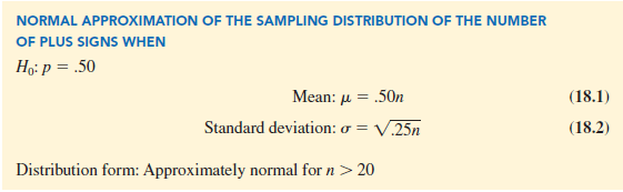
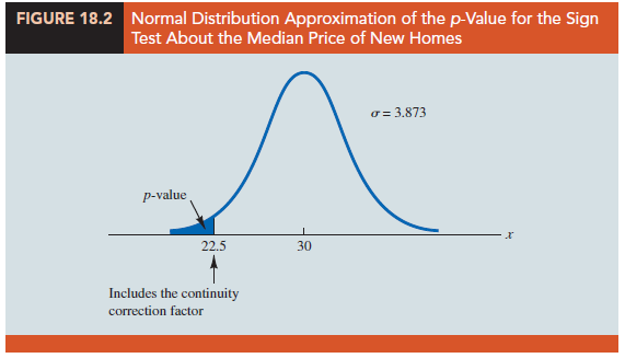
Using equations (18.1) and (18.2) with n = 60 homes and p = .50, the sampling distribution of the number of plus signs can be approximated by a normal distribution with
Let us now use the normal distribution to approximate the binomial probability of 22 or fewer plus signs. Before we proceed, remember that the binomial probability distribution is discrete and the normal probability distribution is continuous. To account for this, the binomial probability of 22 is computed by the normal probability interval 21.5 to 22.5. The .5 added to and subtracted from 22 is called the continuity correction factor. Thus, to compute the p-value for 22 or fewer plus signs we use the normal distribution with m = 30 and s = 3.873 to compute the probability that the normal random variable, x, has a value less than or equal to 22.5. A graph of this p-value is shown in Figure 18.2.
Using this normal distribution, we compute the p-value as follows:
![]()
Using the table of areas for a normal probability distribution, we see that the cumulative probability for z = -1.94 provides the p-value = .0262. With .0262 < .05, we reject the null hypothesis and conclude that the median price of a new home is less than the $236,000 median price a year ago.
Source: Anderson David R., Sweeney Dennis J., Williams Thomas A. (2019), Statistics for Business & Economics, Cengage Learning; 14th edition.
31 Aug 2021
28 Aug 2021
30 Aug 2021
30 Aug 2021
30 Aug 2021
30 Aug 2021