1. Mean
Perhaps the most important measure of location is the mean, or average value, for a variable. The mean provides a measure of central location for the data. If the data are for a sample, the mean is denoted by x; if the data are for a population, the mean is denoted by the Greek letter m.
In statistical formulas, it is customary to denote the value of variable x for the first observation by x1, the value of variable x for the second observation by x2, and so on. In general, the value of variable x for the ,th observation is denoted by x,. For a sample with n observations, the formula for the sample mean is as follows.
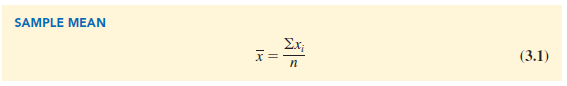
In the preceding formula, the numerator is the sum of the values of the n observations. That is,
![]()
To illustrate the computation of a sample mean, let us consider the following class size data for a sample of five college classes.
![]()
We use the notation x1, x2, x3, x4, x5 to represent the number of students in each of the five classes.
![]()
Hence, to compute the sample mean, we can write
![]()
The sample mean class size is 44 students.
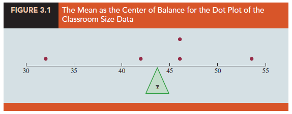
To provide a visual perspective of the mean and to show how it can be influenced by extreme values, consider the dot plot for the class size data shown in Figure 3.1. Treating the horizontal axis used to create the dot plot as a long narrow board in which each of the dots has the same fixed weight, the mean is the point at which we would place a fulcrum or pivot point under the board in order to balance the dot plot. This is the same principle by which a see-saw on a playground works, the only difference being that the see-saw is pivoted in the middle so that as one end goes up, the other end goes down. In the dot plot we are locating the pivot point based upon the location of the dots. Now consider what happens to the balance if we increase the largest value from 54 to 114. We will have to move the fulcrum under the new dot plot in a positive direction in order to reestablish balance. To determine how far we would have to shift the fulcrum, we simply compute the sample mean for the revised class size data.

Thus, the mean for the revised class size data is 56, an increase of 12 students. In other words, we have to shift the balance point 12 units to the right to establish balance under the new dot plot.
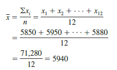
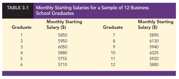
Another illustration of the computation of a sample mean is given in the following situation. Suppose that a college placement office sent a questionnaire to a sample of business school graduates requesting information on monthly starting salaries. Table 3.1 shows the collected data. The mean monthly starting salary for the sample of 12 business college graduates is computed as
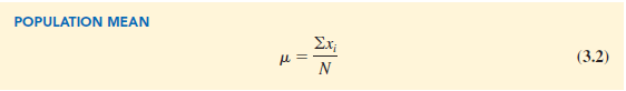
Equation (3.1) shows how the mean is computed for a sample with n observations. The formula for computing the mean of a population remains the same, but we use different notation to indicate that we are working with the entire population. The number of observations in a population is denoted by N and the symbol for a population mean is μ.
2. Weighted Mean
In the formulas for the sample mean and population mean, each x, is given equal importance or weight. For instance, the formula for the sample mean can be written as follows:

This shows that each observation in the sample is given a weight of 1/n. Although this practice is most common, in some instances the mean is computed by giving each observation a weight that reflects its relative importance. A mean computed in this manner is referred to as a weighted mean. The weighted mean is computed as follows:
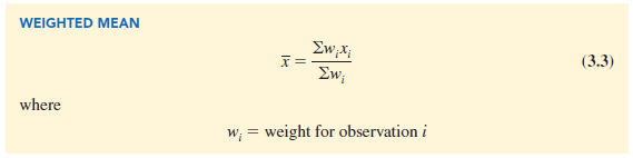
When the data are from a sample, equation (3.3) provides the weighted sample mean. If the data are from a population, m replaces X and equation (3.3) provides the weighted population mean.
As an example of the need for a weighted mean, consider the following sample of five purchases of a raw material over the past three months.
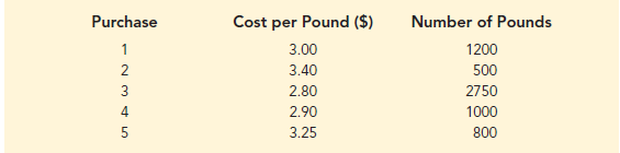
Note that the cost per pound varies from $2.80 to $3.40, and the quantity purchased varies from 500 to 2750 pounds. Suppose that a manager wanted to know the mean cost per pound of the raw material. Because the quantities ordered vary, we must use the formula for a weighted mean. The five cost-per-pound data values are X4 = 3.00, X2= 3.40, X3 = 2.80, X4 = 2.90, and X5 = 3.25. The weighted mean cost per pound is found by weighting each cost by its corresponding quantity. For this example, the weights are w1 = 1200, w2 = 500, w3 = 2750, w4 = 1000, and w5 = 800. Based on equation (3.3), the weighted mean is calculated as follows:
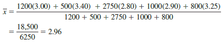
Thus, the weighted mean computation shows that the mean cost per pound for the raw material is $2.96. Note that using equation (3.1) rather than the weighted mean formula in equation (3.3) would provide misleading results. In this case, the sample mean of the five cost-per-pound values is (3.00 + 3.40 + 2.80 + 2.90 + 3.25)/5 = 15.35/5 = $3.07, which overstates the actual mean cost per pound purchased.
The choice of weights for a particular weighted mean computation depends upon the application. An example that is well known to college students is the computation of a grade point average (GPA). In this computation, the data values generally used are 4 for an A grade, 3 for a B grade, 2 for a C grade, 1 for a D grade, and 0 for an F grade. The weights are the number of credit hours earned for each grade. In other weighted mean computations, quantities such as pounds, dollars, or volume are frequently used as weights. In any case, when observations vary in importance, the analyst must choose the weight that best reflects the importance of each observation in the determination of the mean.
3. Median
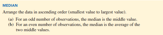
The median is another measure of central location. The median is the value in the middle when the data are arranged in ascending order (smallest value to largest value). With an odd number of observations, the median is the middle value. An even number of observations has no single middle value. In this case, we follow convention and define the median as the average of the values for the middle two observations. For convenience the definition of the median is restated as follows.
Let us apply this definition to compute the median class size for the sample of five college classes. Arranging the data in ascending order provides the following list.
32 42 46 46 54
Because n = 5 is odd, the median is the middle value. Thus the median class size is 46 students. Even though this data set contains two observations with values of 46, each observation is treated separately when we arrange the data in ascending order.
Suppose we also compute the median starting salary for the 12 business college graduates in Table 3.1. We first arrange the data in ascending order.
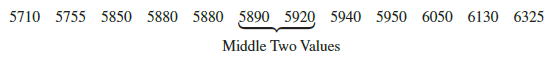
Because n = 12 is even, we identify the middle two values: 5890 and 5920. The median is the average of these values.
![]()
The procedure we used to compute the median depends upon whether there is an odd number of observations or an even number of observations. Let us now describe a more conceptual and visual approach using the monthly starting salary for the 12 business college graduates. As before, we begin by arranging the data in ascending order.
5710 5755 5850 5880 5880 5890 5920 5940 5950 6050 6130 6325
Once the data are in ascending order, we trim pairs of extreme high and low values until no further pairs of values can be trimmed without completely eliminating all the data. For instance, after trimming the lowest observation (5710) and the highest observation (6325) we obtain a new data set with 10 observations.
![]()
We then trim the next lowest remaining value (5755) and the next highest remaining value (6130) to produce a new data set with eight observations.
![]()
Continuing this process, we obtain the following results.
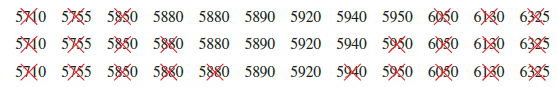
At this point no further trimming is possible without eliminating all the data. So, the median is just the average of the remaining two values. When there is an even number of observations, the trimming process will always result in two remaining values, and the average of these values will be the median. When there is an odd number of observations, the trimming process will always result in one final value, and this value will be the median. Thus, this method works whether the number of observations is odd or even.
Although the mean is the more commonly used measure of central location, in some situations the median is preferred. The mean is influenced by extremely small and large data values. For instance, suppose that the highest paid graduate (see Table 3.1) had a starting salary of $15,000 per month. If we change the highest monthly starting salary in Table 3.1 from $6325 to $15,000 and recompute the mean, the sample mean changes from $5940 to $6663. The median of $5905, however, is unchanged, because $5890 and $5920 are still the middle two values. With the extremely high starting salary included, the median provides a better measure of central location than the mean. We can generalize to say that whenever a data set contains extreme values, the median is often the preferred measure of central location.
4. Geometric Mean
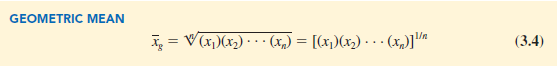
The geometric mean is a measure of location that is calculated by finding the nth root of the product of n values. The general formula for the geometric mean, denoted Xg, follows.
The geometric mean is often used in analyzing growth rates in financial data. In these types of situations the arithmetic mean or average value will provide misleading results.
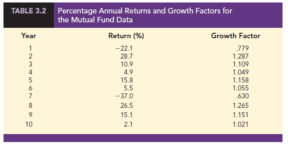
To illustrate the use of the geometric mean, consider Table 3.2, which shows the percentage annual returns, or growth rates, for a mutual fund over the past 10 years. Suppose we want to compute how much $100 invested in the fund at the beginning of year 1 would be worth at the end of year 10. Let’s start by computing the balance in the fund at the end of year 1. Because the percentage annual return for year 1 was -22.1%, the balance in the fund at the end of year 1 would be
$100 – .221($100) = $100(1 – .221) = $100(.779) = $77.90
We refer to .779 as the growth factor for year 1 in Table 3.2. We can compute the balance at the end of year 1 by multiplying the value invested in the fund at the beginning of year 1 times the growth factor for year 1: $100(.779) = $77.90.
The balance in the fund at the end of year 1, $77.90, now becomes the beginning balance in year 2. So, with a percentage annual return for year 2 of 28.7%, the balance at the end of year 2 would be
$77.90 + .287($77.90) = $77.90(1 + .287) = $77.90(1.287) = $100.2573
Note that 1.287 is the growth factor for year 2. And, by substituting $100(.779) for $77.90 we see that the balance in the fund at the end of year 2 is
$100(.779)(1.287) = $100.2573
In other words, the balance at the end of year 2 is just the initial investment at the beginning of year 1 times the product of the first two growth factors. This result can be generalized to show that the balance at the end of year 10 is the initial investment times the product of all 10 growth factors.
$100[(.779)(1.287)(1.109)(1.049)(1.158)(1.055)(.630)(1.265)(1.151)(1.021)] =
$100(1.334493) = $133.4493
So, a $100 investment in the fund at the beginning of year 1 would be worth $133.4493 at the end of year 10. Note that the product of the 10 growth factors is 1.334493. Thus, we can compute the balance at the end of year 10 for any amount of money invested at the beginning of year 1 by multiplying the value of the initial investment times 1.334493. For instance, an initial investment of $2500 at the beginning of year 1 would be worth $2500(1.334493) or approximately $3336 at the end of year 10.
What was the mean percentage annual return or mean rate of growth for this investment over the 10-year period? The geometric mean of the 10 growth factors can be used to answer to this question. Because the product of the 10 growth factors is 1.334493, the geometric mean is the 10th root of 1.334493 or
![]()
The geometric mean tells us that annual returns grew at an average annual rate of (1.029275 – 1)100% or 2.9275%. In other words, with an average annual growth rate of 2.9275%, a $100 investment in the fund at the beginning of year 1 would grow to $100(1.029275)10 = $133.4493 at the end of 10 years.
It is important to understand that the arithmetic mean of the percentage annual returns does not provide the mean annual growth rate for this investment. The sum of the 10 annual percentage returns in Table 3.2 is 50.4. Thus, the arithmetic mean of the 10 percentage annual returns is 50.4/10 = 5.04%. A broker might try to convince you to invest in this fund by stating that the mean annual percentage return was 5.04%. Such a statement is not only misleading, it is inaccurate. A mean annual percentage return of 5.04% corresponds to an average growth factor of 1.0504. So, if the average growth factor were really 1.0504, $100 invested in the fund at the beginning of year 1 would have grown to $100(1.0504)10 = $163.51 at the end of 10 years. But, using the 10 annual percentage returns in Table 3.2, we showed that an initial $100 investment is worth $133.45 at the end of 10 years. The broker’s claim that the mean annual percentage return is 5.04% grossly overstates the true growth for this mutual fund. The problem is that the sample mean is only appropriate for an additive process. For a multiplicative process, such as applications involving growth rates, the geometric mean is the appropriate measure of location.
While the applications of the geometric mean to problems in finance, investments, and banking are particularly common, the geometric mean should be applied any time you want to determine the mean rate of change over several successive periods. Other common applications include changes in populations of species, crop yields, pollution levels, and birth and death rates. Also note that the geometric mean can be applied to changes that occur over any number of successive periods of any length. In addition to annual changes, the geometric mean is often applied to find the mean rate of change over quarters, months, weeks, and even days.
5. Mode
Another measure of location is the mode. The mode is defined as follows.
To illustrate the identification of the mode, consider the sample of five class sizes.
The only value that occurs more than once is 46. Because this value, occurring with a frequency of 2, has the greatest frequency, it is the mode. As another illustration, consider the sample of starting salaries for the business school graduates. The only monthly starting salary that occurs more than once is $5880. Because this value has the greatest frequency, it is the mode.
Situations can arise for which the greatest frequency occurs at two or more different values. In these instances more than one mode exist. If the data contain exactly two modes, we say that the data are bimodal. If data contain more than two modes, we say that the data are multimodal. In multimodal cases the mode is almost never reported because listing three or more modes would not be particularly helpful in describing a location for the data.
6. Percentiles
A percentile provides information about how the data are spread over the interval from the smallest value to the largest value. For a data set containing n observations, the pth percentile divides the data into two parts: approximately p% of the observations are less than the pth percentile, and approximately (100 – p)% of the observations are greater than the pth percentile.
Colleges and universities frequently report admission test scores in terms of percentiles. For instance, suppose an applicant obtains a score of 630 on the math portion of an admission test. How this applicant performed in relation to others taking the same test may not be readily apparent from this score. However, if the score of 630 corresponds to the 82nd percentile, we know that approximately that 82% of the applicants scored lower than this individual and approximately 18% of the applicants scored higher than this individual.
To calculate the pth percentile for a data set containing n observations, we must first arrange the data in ascending order (smallest value to largest value). The smallest value is in position 1, the next smallest value is in position 2, and so on. The location of the pth percentile, denoted Lp, is computed using the following equation:
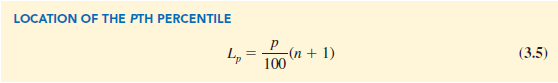
Once we find the position of the value of the pth percentile, we have the information we need to calculate the pth percentile.
To illustrate the computation of the pth percentile, let us compute the 80th percentile for the starting salary data in Table 3.1. We begin by arranging the sample of 12 starting salaries in ascending order.

The position of each observation in the sorted data is shown directly below its value. For instance, the smallest value (5710) is in position 1, the next smallest value (5755) is in position 2, and so on. Using equation (3.5) with p = 80 and n = 12, the location of the 80th percentile is
![]()
The interpretation of L80 = 10.4 is that the 80th percentile is 40% of the way between the value in position 10 and the value in position 11. In other words, the 80th percentile is the value in position 10 (6050) plus .4 times the difference between the value in position 11 (6130) and the value in position 10 (6050). Thus, the 80th percentile is
80th percentile = 6050 + .4(6130 – 6050) = 6050 + .4(80) = 6082
Let us now compute the 50th percentile for the starting salary data. With p = 50 and n = 12, the location of the 50th percentile is
![]()
With L50 = 6.5, we see that the 50th percentile is 50% of the way between the value in position 6 (5890) and the value in position 7 (5920). Thus, the 50th percentile is
50th percentile = 5890 + .5(5920 – 5890) = 5890 + .5(30) = 5905
Note that the 50th percentile is also the median.
7. Quartiles
It is often desirable to divide a data set into four parts, with each part containing approximately one-fourth, or 25%, of the observations. These division points are referred to as the quartiles and are defined as follows.
Q1 = first quartile, or 25th percentile
Q2 = second quartile, or 50th percentile (also the median)
Q3 = third quartile, or 75th percentile
Because quartiles are specific percentiles, the procedure for computing percentiles can be used to compute the quartiles.
To illustrate the computation of the quartiles for a data set consisting of n observations, we will compute the quartiles for the starting salary data in Table 3.1. Previously we showed that the 50th percentile for the starting salary data is 5905; thus, the second quartile (median) is Q2 = 5905. To compute the first and third quartiles, we must find the 25th and 75th percentiles. The calculations follow.
For Q1
![]()
The first quartile, or 25th percentile, is .25 of the way between the value in position 3 (5850) and the value in position 4 (5880). Thus,
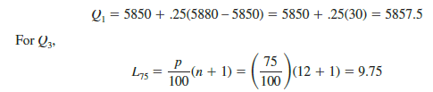
The third quartile, or 75th percentile, is .75 of the way between the value in position 9 (5950) and the value in position 10 (6050). Thus,
Q3 = 5950 + .75(6050 – 5950) = 5950 + .75(100) = 6025
The quartiles divide the starting salary data into four parts, with each part containing 25% of the observations.
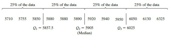
We defined the quartiles as the 25th, 50th, and 75th percentiles and then we computed the quartiles in the same way as percentiles. However, other conventions are sometimes used to compute quartiles, and the actual values reported for quartiles may vary slightly depending on the convention used. Nevertheless, the objective of all procedures for computing quartiles is to divide the data into four parts that contain equal numbers of observations.
Source: Anderson David R., Sweeney Dennis J., Williams Thomas A. (2019), Statistics for Business & Economics, Cengage Learning; 14th edition.
30 Aug 2021
30 Aug 2021
30 Aug 2021
30 Aug 2021
30 Aug 2021
30 Aug 2021