Calculating the Probability of Type II Errors

In this section we show how to calculate the probability of making a Type II error for a hypothesis test about a population mean. We illustrate the procedure by using the lot- acceptance example described in Section 9.6. The null and alternative hypotheses about the mean number of hours of useful life for a shipment of batteries are H₀: μ ≥ 120 and H_a: μ ≤ 120. If H₀ is rejected, the decision will be to return the shipment to the supplier because the mean hours of useful life are less than the specified 120 hours. If H₀ is not rejected, the decision will be to accept the shipment.

Suppose a level of significance of a = .05 is used to conduct the hypothesis test. The test statistic in the s known case is

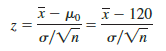
Based on the critical value approach and z.₀₅ = 1.645, the rejection rule for the lower tail test is

Suppose a sample of 36 batteries will be selected and based upon previous testing the population standard deviation can be assumed known with a value of s = 12 hours. The rejection rule indicates that we will reject H₀ if

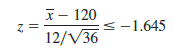
Solving for x in the preceding expression indicates that we will reject H0 if

Rejecting H0 when x ≤ 116.71 means that we will make the decision to accept the shipment whenever

With this information, we are ready to compute probabilities associated with making a Type II error. First, recall that we make a Type II error whenever the true shipment mean is less than 120 hours and we make the decision to accept H0: μ ≥ 120. Hence, to compute the probability of making a Type II error, we must select a value of m less than 120 hours. For example, suppose the shipment is considered to be of poor quality if the batteries have a mean life of μ = 112 hours. If μ = 112 is really true, what is the probability of accepting H0: μ ≥ 120 and hence committing a Type II error? Note that this probability is the probability that the sample mean x is greater than 116.71 when m = 112. Figure 9.8 shows the sampling distribution of x when the mean is μ = 112. The shaded area in the upper tail gives the probability of obtaining x > 116.71. Using the standard normal distribution, we see that at x = 116.71

The standard normal probability table shows that with z = 2.36, the area in the upper tail is 1.0000 − .9909 = .0091. Thus, .0091 is the probability of making a Type II error when μ = 112. Denoting the probability of making a Type II error as b, we see that when μ = 112, β = .0091. Therefore, we can conclude that if the mean of the population is 112 hours, the probability of making a Type II error is only .0091.

We can repeat these calculations for other values of μ less than 120. Do ing so will show a different probability of making a Type II error for each value of μ. For example, supposethe shipment of batteries has a  mean useful life of μ = 115 hours. Because we will accept H0 whenever x > 116.71, the z value for μ = 115 is given by

From the standard normal probability table, we find that the area in the upper tail of the standard normal distribution for z = .86 is 1.0000 – .8051 = .1949. Thus, the probability of making a Type II error is β = .1949 when the true mean is μ = 115.

In Table 9.5 we show the probability of making a Type II error for a variety of values of m less than 120. Note that as μ increases toward 120, the probability of making a Type II error increases toward an upper bound of .95. However, as μ decreases to values farther below 120, the probability of making a Type II error diminishes. This pattern is what we should expect. When the true population mean m is close to the null hypothesis value of μ = 120, the probability is high that we will make a Type II error. However, when the true population mean m is far below the null hypothesis value of μ = 120, the probability is low that we will make a Type II error.

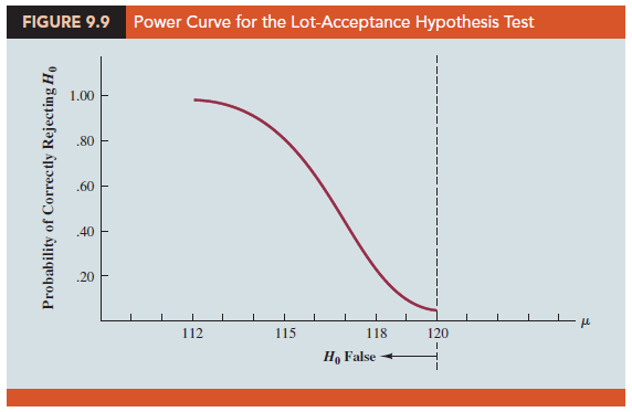
The probability of correctly rejecting H₀ when it is false is called the power of the test. For any particular value of m, the power is 1 – b; that is, the probability of correctly rejecting the null hypothesis is 1 minus the probability of making a Type II error. Values of power are also listed in Table 9.5. On the basis of these values, the power associated with each value of m is shown graphically in Figure 9.9. Such a graph is called a power curve. Note that the power curve extends over the values of m for which the null hypothesis is false. The height of the power curve at any value of m indicates the probability of correctly rejecting H₀ when H₀ is false.

In summary, the following step-by-step procedure can be used to compute the probabil­ity of making a Type II error in hypothesis tests about a population mean.

1. Formulate the null and alternative hypotheses.
2. Use the level of significance a and the critical value approach to determine the critical value and the rejection rule for the test.
3. Use the rejection rule to solve for the value of the sample mean corresponding to the critical value of the test statistic.
4. Use the results from step 3 to state the values of the sample mean that lead to the acceptance of H₀. These values define the acceptance region for the test.
5. Use the sampling distribution of x for a value of m satisfying the alternative hypothe­sis, and the acceptance region from step 4, to compute the probability that the sample mean will be in the acceptance region. This probability is the probability of making a Type II error at the chosen value of μ.

Source:  Anderson David R., Sweeney Dennis J., Williams Thomas A. (2019), Statistics for Business & Economics, Cengage Learning; 14th edition.