In Section 14.8 we showed how residual analysis could be used to determine when violations of assumptions about the regression model occur. In this section, we discuss how residual analysis can be used to identify observations that can be classified as outliers or as being especially influential in determining the estimated regression equation. Some steps that should be taken when such observations occur are discussed.
1. Detecting Outliers
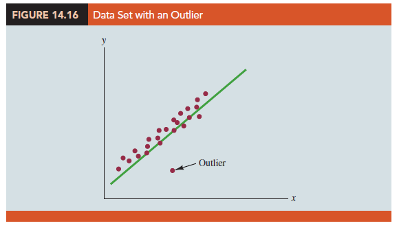
Figure 14.16 is a scatter diagram for a data set that contains an outlier, a data point (observation) that does not fit the trend shown by the remaining data. Outliers represent observations that are suspect and warrant careful examination. They may represent erroneous data; if so, the data should be corrected. They may signal a violation of model assumptions; if so, another model should be considered. Finally, they may simply be unusual values that occurred by chance. In this case, they should be retained.
To illustrate the process of detecting outliers, consider the data set in Table 14.11;
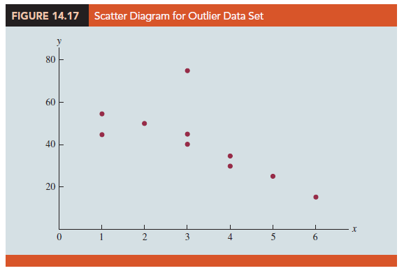
Figure 14.17 is a scatter diagram. Except for observation 4 (x4 = 3, y4 = 75), a pattern suggesting a negative linear relationship is apparent. Indeed, given the pattern of the rest of the data, we would expect y4 to be much smaller and hence would identify the corresponding observation as an outlier. For the case of simple linear regression, one can often detect outliers by simply examining the scatter diagram.
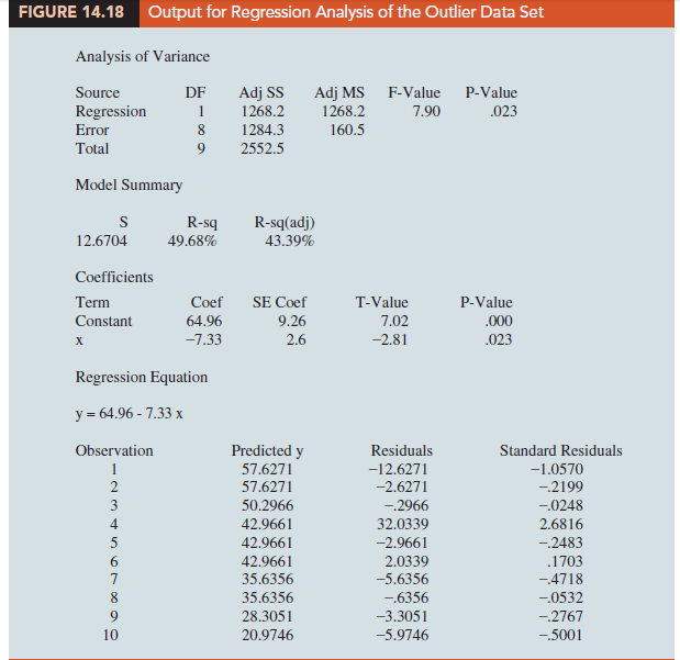
The standardized residuals can also be used to identify outliers. If an observation deviates greatly from the pattern of the rest of the data (e.g., the outlier in Figure 14.16), the corresponding standardized residual will be large in absolute value. Many computer packages automatically identify observations with standardized residuals that are large in absolute value. For the data in Table 14.11, Figure 14.18 shows the output from a regression analysis, including the regression equation, the predicted values of y, the residuals, and the standardized residuals. The highlighted portion of the output shows that the standardized residual for observation 4 is 2.67. With normally distributed errors, standardized residuals should be outside the range of -2 to +2 approximately 5% of the time.
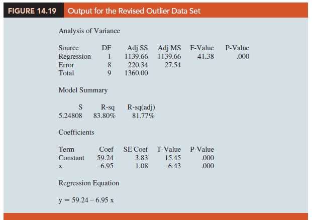
In deciding how to handle an outlier, we should first check to see whether it is a valid observation. Perhaps an error was made in initially recording the data or in entering the data into the computer file. For example, suppose that in checking the data for the outlier in Table 14.11, we find an error; the correct value for observation 4 is x4 = 3, y4 = 30. Figure 14.19 is a portion of the output obtained after correction of the value of y4. We see that using the incorrect data value substantially affected the goodness of fit. With the correct data, the value of R-sq increased from 49.68% to 83.8% and the value of b0 decreased from 64.96 to 59.24. The slope of the line changed from -7.33 to -6.95.
The identification of the outlier enabled us to correct the data error and improve the regression results.
2. Detecting Influential Observations
Sometimes one or more observations exert a strong influence on the results obtained.
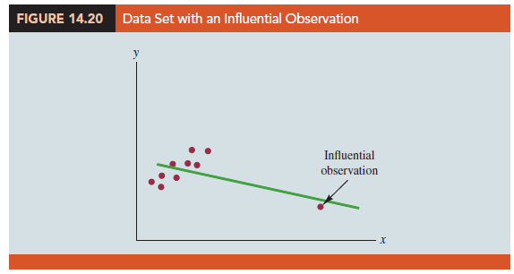
Figure 14.20 shows an example of an influential observation in simple linear regression. The estimated regression line has a negative slope. However, if the influential observation were dropped from the data set, the slope of the estimated regression line would change from negative to positive and the y-intercept would be smaller. Clearly, this one observation is much more influential in determining the estimated regression line than any of the others; dropping one of the other observations from the data set would have little effect on the estimated regression equation.
Influential observations can be identified from a scatter diagram when only one independent variable is present. An influential observation may be an outlier (an observation with a y value that deviates substantially from the trend), it may correspond to an x value far away from its mean (e.g., see Figure 14.20), or it may be caused by a combination of the two (a somewhat off-trend y value and a somewhat extreme x value).
Because influential observations may have such a dramatic effect on the estimated regression equation, they must be examined carefully. We should first check to make sure that no error was made in collecting or recording the data. If an error occurred, it can be corrected and a new estimated regression equation can be developed. If the observation is valid, we might consider ourselves fortunate to have it. Such a point, if valid, can contribute to a better understanding of the appropriate model and can lead to a better estimated regression equation. The presence of the influential observation in Figure 14.20, if valid, would suggest trying to obtain data on intermediate values of x to understand better the relationship between x and y.
Observations with extreme values for the independent variables are called high leverage points. The influential observation in Figure 14.20 is a point with high leverage. The leverage of an observation is determined by how far the values of the independent variables are from their mean values. For the single-independent-variable case, the leverage of the ith observation, denoted h, can be computed by using equation (14.33).
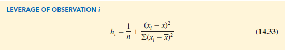
From the formula, it is clear that the farther xi is from its mean X, the higher the leverage of observation i.
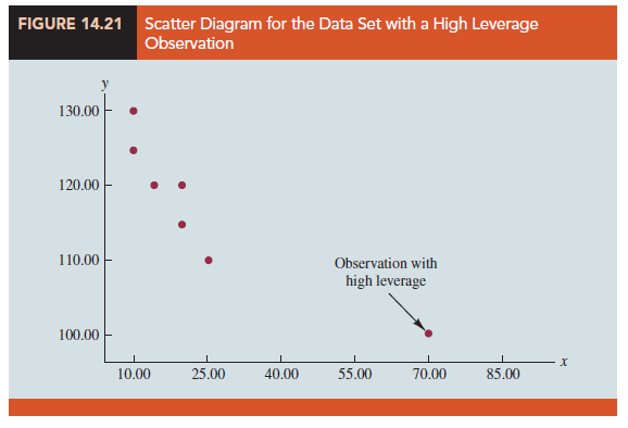
Many statistical packages automatically identify observations with high leverage as part of the standard regression output. As an illustration of points with high leverage, let us consider the data set in Table 14.12.
From Figure 14.21, a scatter diagram for the data set in Table 14.12, it is clear that observation 7 (x = 70, y = 100) is an observation with an extreme value of x. Hence, we would expect it to be identified as a point with high leverage. For this observation, the leverage is computed by using equation (14.33) as follows.
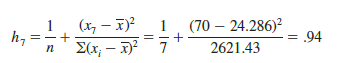
For the case of simple linear regression, observations have high leverage if ht > 6/n or .99, whichever is smaller. For the data set in Table 14.12, 6/n = 6/7 = .86. Because h 7 = .94 > .86, we will identify observation 7 as an observation whose x value gives it large influence.
Influential observations that are caused by an interaction of large residuals and high leverage can be difficult to detect. Diagnostic procedures are available that take both into account in determining when an observation is influential. One such measure, called Cook’s D statistic, will be discussed in Chapter 15.
Source: Anderson David R., Sweeney Dennis J., Williams Thomas A. (2019), Statistics for Business & Economics, Cengage Learning; 14th edition.
28 Aug 2021
30 Aug 2021
31 Aug 2021
31 Aug 2021
28 Aug 2021
31 Aug 2021