Time-Varying Volatility and ARCH Models by using EViews: An Introduction to Financial Econometrics

1. TIME-VARYING VOLATILITY

In this chapter we are concerned with variances that change over time, i.e., time-varying variance processes. The model we focus on is called the AutoRegressive Conditional Heteroskedastic (ARCH) model.

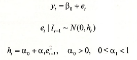
This is an example of an ARCH(l) model since the time varying variance h_t is a function of a constant term (a₀) plus a term lagged once, the square of the error in the previous period ( cqe,².,). The coefficients, a₀ and a,, have to be positive to ensure a positive variance. The coefficient a, must be less than 1, otherwise h_t will continue to increase over time, eventually exploding.

Conditional normality means that the distribution is a function of known information at time t -1i.e., when t = 2, (e₂ | I₁,) ~ N(0,a₀ + a₁e₁²) and so on.

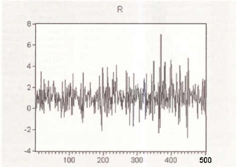
The EViews workfile byd.wfl contains the returns to BrightenYourDayLighting. To plot the times series, double-click the variable and select View/ Open Graph/ Line & symbol and click OK.

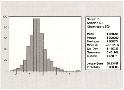
To generate the histogram, select View/ Descriptive Statistics & Tests/ Histogram and Stats.

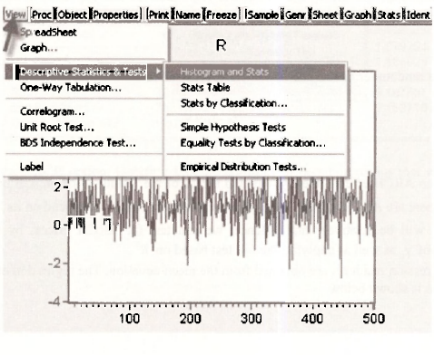
Clicking this option gives the distribution below.

2. TESTING FOR ARCH EFFECTS

To test For first order ARCH, regress the squared regression residuals e² on their lags e²_t-1:

where v, is a random term. The null and alternative hypotheses are:

If there are no ARCH effects, then y₁ = 0 and the fit of the testing equation will be poor with a low R². If there are ARCH effects, we expect the magnitude of e² to depend on its lagged values and the R² will be relatively high. Hence, we can test For ARCH effects by checking the significance of y₁, as well as applying the LMtest based on R².

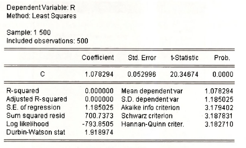
The regression residuals are obtained from the mean equation. The regression of returns on a constant term is shown below.

To generate the regression residuals, select View, select Residual Tests/Heteroskedasticity Tests from the drop down menus.

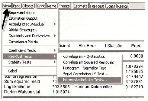
Then select the ARCH option. Inserting 1 in the Number of lags box means that we are testing for ARCH( 1) effects.

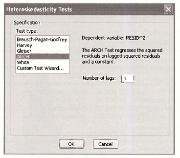
Clicking on OK gives the ARCH test results below.

Since the CM statistic (62.159) is significant, we reject the null hypothesis that there is no first- order ARCH effects. Note that the LM statistic in EViews is calculated as LM = TxR² = 499×0.124568=62.16. Furthermore, the F- and t-statistics (62.16 = 8.4095²) corroborate the presence of first order ARCH effects.

3. ESTIMATING AN ARCH MODEL

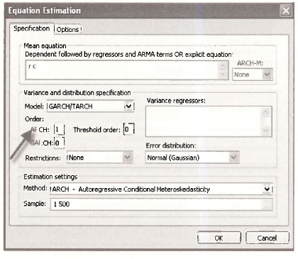
To estimate an ARCH model, click Quick/ Estimate equation and select the ARCH option from the drop-down menu in Method.

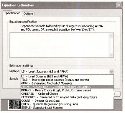
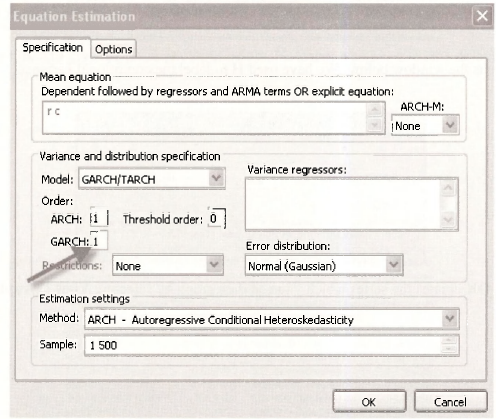
A screen with an upper Mean equation and a lower Variance and distribution specification section will open up. In the mean equation section, enter the regression of the returns, R, on a constant, C. In the variance and distribution specification section, to estimate an ARCH model of order 1, type a 1 against ARCH.

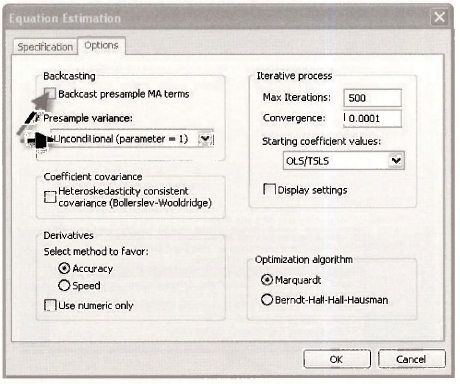
To obtain the standard errors reported in the text, click on Options (top left hand comer) and then pick the options noted below. As discussed in the text, time series models require an initial starting value, in this case the initial variance h.. The options suggested here set the initial variance to the unconditional sample variance.

Clicking on OK will give the EViews output below. Note that we have used the default Marquardt algorithm to generate these results.

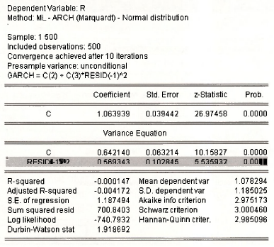
The top section is the mean equation. It shows that the average return is 1.063939. The lower section is the variance equation that gives the result of the ARCH model, namely, that the time varying volatility h_t includes a constant component (0.642140) plus a component which depends on past errors. The shaded line highlights the significant ARCH effects.

To generate the conditional variance series shown in the text, click on Proc and select Make GARCH Variance Series from the drop-down menu.

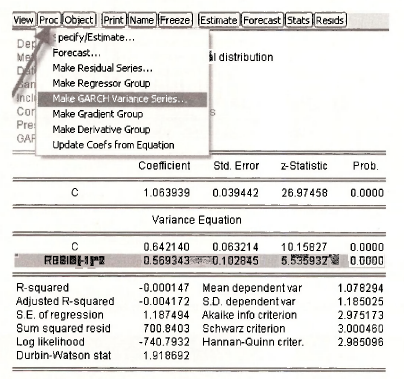
Clicking opens the window below. We have used H to label the conditional variance.

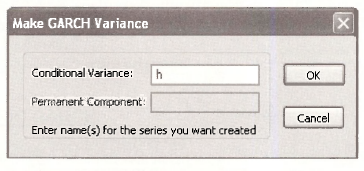
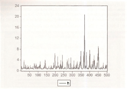
Clicking on OK creates the series which you can then graph by selecting View / Graph/ Line & Symbol/.

4. GENERALIZED ARCH

To estimate a GARCH(1,1) model, select the option shown below.

Clicking on OK produces the EViews results below.

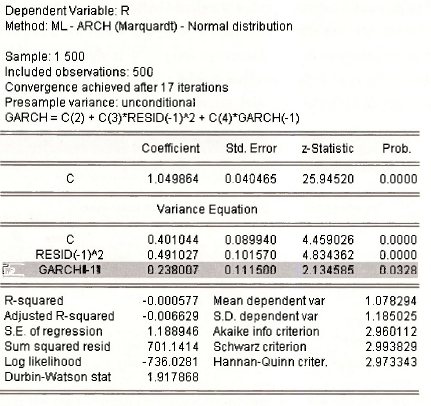
Recall that the generalized GARCH(1,1) model is of the form:

We also note that we need a₁ + β₁ < 1 for stationarity; if a₁ + β₁ > 1 we have a so-called “integrated GARCH” process, or IGARCH.

The shaded line in the EViews output shows the significance of the GARCH term. These results show that the volatility coefficients, the one in front of the ARCH effect (0.491027) and the one in front of the GARCH effect (0.238007) are both positive and their sum is between zero and one, as required by theory.

5. ASYMMETRIC GARCH

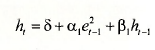
The threshold ARCH model, or T-ARCH, is one example where positive and negative news are treated asymmetrically. In the T-GARCH version of the model, the specification of the conditional variance is:

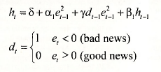
where y is known as the asymmetry or leverage term.

When y = 0, the model collapses to the standard GARCH form. Otherwise, when the shock is positive (i.e. good news) the effect on volatility is a, but when the news is negative (i.e. bad news) the effect on volatility is a, + y . Hence, so long as y is significant and positive, negative shocks have a larger effect on h_t than positive shocks.

To estimate a threshold GARCH model, select the option shown below.

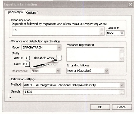
Clicking OK gives the EViews ouput

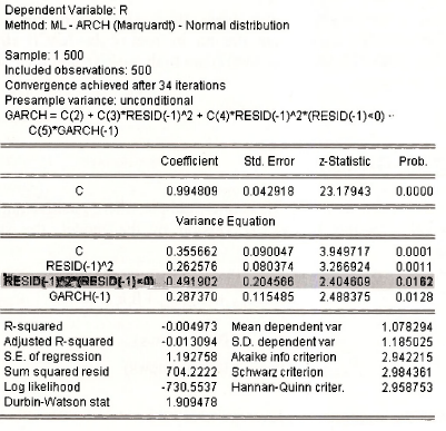
Since the coefficient on the asymmetric term (0.492) is significant, we infer that there is evidence that positive and negative shocks have different effects. In particular, when the shock is positive, the estimate of the time-varying volatility is

and when the shock is negative, the estimate of the time-varying volatility is

6. GARCH-IN-MEAN

The equations of a GARCH-in-mean model are shown below:

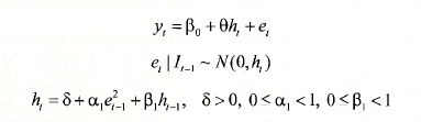
The first equation is the mean equation; it now shows the effect of the conditional variance on the dependent variable. In particular, note that the model postulates that the conditional variance h_t affects y_t by a factor 0. The other two equations are as before.

To estimate a GARCH in mean model, select the option shown below.

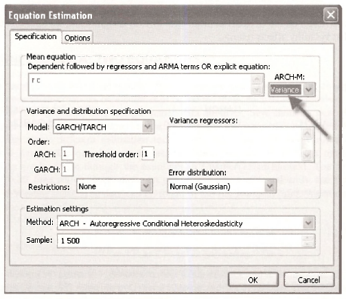
Clicking on OK produces the EViews ouput below.

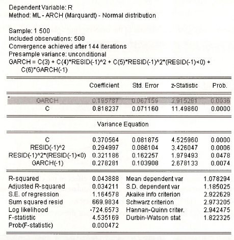
Since the coefficient on the GARCH in mean term (0.196) is significant, we infer that there evidence that volatility affects returns.

Source: Griffiths William E., Hill R. Carter, Lim Mark Andrew (2008), Using EViews for Principles of Econometrics, John Wiley & Sons; 3rd Edition.