Panel Data Models by using EViews

1. GRUNFELD DATA: TWO EQUATIONS

Panel data are data with two dimensions, a time dimension and a cross-section dimension. They typically comprise observations on a number of economic units, such as individuals or firms, over a number of time periods. The use of panel data involves new models, new econometric techniques and new ways of handling the data. EViews has the capacity to estimate a vast array of models, using many different estimation techniques. Also, the user has various options for handling the data and proceeding to estimation. Some but not all of those options will be introduced as we lead you through the examples in Chapter 15 of the text. The first example involves T = 20 time series observations on just N = 2 cross sectional units, the firms General Electric and Westinghouse. The data can be found in the file grunfeld2.dat. We are interested in estimating the two equations

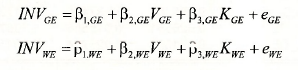
where INV denotes investment, V denotes market value of stock and K denotes capital stock, with the subscripts GE and WE referring to General Electric and Westinghouse, respectively. There are various ways of estimating these two equations depending on what further assumptions are made about the coefficients and the error terms in each of the equations. We first consider separate least squares estimation of each equation.

1.1. Separate least squares estimation

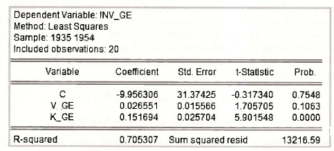
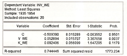
In the following screenshot the two separate equation specifications for the GE and WE equations have been superimposed on the workfile. There is nothing new in these specifications. They are straightforward least squares estimations. With respect to the structure of the workfile, there are two things worth noting. First, the observations are dated with the range and sample specified as annual data from 1935 to 1954. Second, each of the variables has a “subscript”, GE or _WE to signify whether the observations are for General Electric or Westinghouse. These “subscripts” are known as cross section identifiers. They will be important in subsequent sections of this chapter.

The outputs from each of these regressions follow. Note that they confirm the results in Table 15.1 on page 386 of the text.

1.2. Stacking the data

In the previous section we estimated two regression equations with 20 observations for each. As noted in equation (15.6) of the text, the same least squares estimates can be obtained by pooling the observations into one sample of 40, and including intercept and slope dummy variables for each of the coefficients. The standard errors turn out differently, however. With separate least squares estimation we get separate estimates for a²_CE and a²_WE . When the observations are pooled into one sample, the implicit assumption is that a²_GE = a²_VE and only one error variance estimate is obtained.

To obtain the pooled dummy variable estimates, it is convenient to stack the observations into one sample of size 40. In addition to stacking INV, V and K, we will create the required dummy variable by defining DUM WE = 1 and DUM_GE = 0, and also stacking these two series.

series dum we = 1

series dum_ge = 0

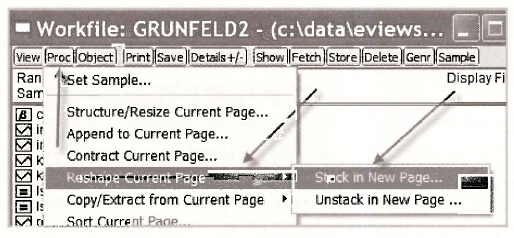
We have chosen the notation DUM rather than D as used by the text because EViews reserves D to be used as a difference operator, as was described in Chapter 12. Stacking is carried out by creating a second page in our workfile and storing the stacked series in that page. But, first we name the first page that contains the unstacked data. Go to fProcl, and select Rename Current Page. In the resulting dialog box, call the page unstacked.

To create a new page with the stacked data, go to Proc/Reshape Current Page/Stack in New Page.

A Workflle Stack dialog box appears. The cross section identifiers _GE and _WE are inserted in the Stacking Identifiers box. In the box that says Series to stack into new workflle page, each of the series names is entered without the subscripts (identifiers), and with each identifier replaced by a question mark ?. Leaving the box below that blank will mean that the new series of length 40, with both the GE and WE observations, will be called INV, V, K and DUM.

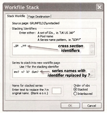
Notice the second tab in the Workfile Stack box called Page Destination. Click on that. We are keeping the current workfile and naming the new page stacked.

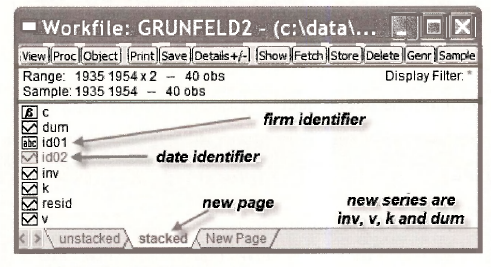
The new workfile page called stacked is illustrated below. Check out the following.

1. The Range is given as 1935 1954 x 2 implying we have two cross sections for the specified time period.
2. The names of the new series that include all 40 observations are INV, V, K and
3. There are two new series ID01 and The first one indicates which observations are GE and which are WE. The second contains the date of each observation.

Open the various series and familiarize yourself with how EViews has set them up.

1.3. Least squares estimation with dummy variables

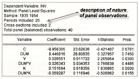
We are now in a position to obtain the estimates given in Table 15.2 on page 387 of the text. Follow the familiar routine of going to Object/New Object/Equation, name the equation object and fill in the Equation specification.

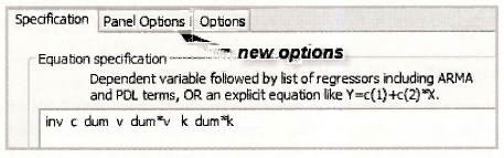
The variables specified are those that appear in equation (15.6) and Table 15.2 of the text. Notice that we are able to enter the products dum*v and dum*k without creating new series. EViews figures it out and gives you the results.

Something new that has suddenly turned up is another tab called Panel Options. Because you went through a stacking procedure, EViews knows that the data are panel data. Accordingly, it set up a panel workfile structure that specifies a panel range and includes objects describing the cross section and time series components. The panel workfile structure includes Panel Options in the Equation Estimation window. For the moment we do not need these options, but we do consider some of them shortly. Clicking OK reveals the results in Table 15.2 on page 387.

1.4. Introducing the pool object

The dummy variable model estimated in the previous section is given by

Using the substitutions

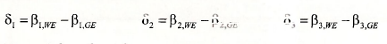
the dummy variable model can be written as

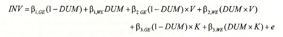
Estimating this equation will give exactly the same results as those from the earlier dummy variable model in the sense that estimates and standard errors of corresponding coefficients will be equal. We can estimate it from the stacked page of grunfeld2.wfl, using the equation specification

inv (1-dum) dum (1-dum)*v dum*v (1-dum)*k dum*k

Try it! See what you get. Can you match corresponding coefficients with Table 15.2?

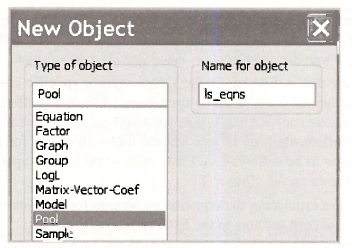
We can also get these estimates using a pool object in the unstacked page. Return to the unstacked page and select Object/New Object/Pool. We named the pool object LS_EQNS.

EViews will then ask you for the cross section identifiers which in this case are GE and WE. For this procedure to work, series names should be expressed with a common component such as INV, K and V and with a cross section identifying component like _GE and WE.

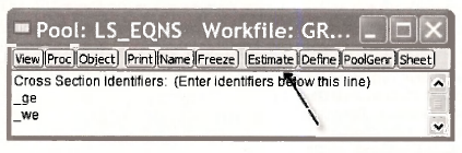
Then click on Estimate. Wow! Look at all the boxes you have to fill in. Don’t be scared. At the moment we are only concerned with two of them.

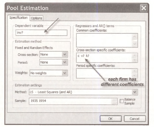
1. For the Dependent variable we have written INV?. Writing it this way, with the question mark, tells EViews to consider all values on investment. Remember that you have already told EViews about the cross-section identifiers. It won’t forget.
2. The other box that is filled in is the Cross-section specific coefficients We chose this one because we want to allow the General Electric coefficients to be different from the Westinghouse coefficients. If you wanted them to be the same, you would choose the Common coefficients box. If you wanted the coefficients for some variables to be the same and some to be different, you can write some of the explanatory variable names in one box and some in the other.
3. Because we are estimating the equation by straightforward least squares, we do not need to change the default settings in the Estimation method

The results follow. They are equivalent to those in Table 15.2, although at first glance you might not think so. We can see the equivalence by noting that

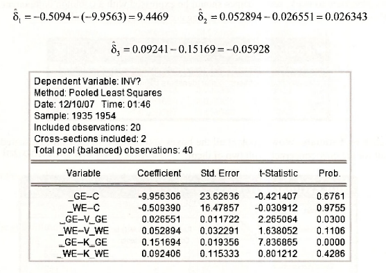
1.5. Seemingly unrelated regressions

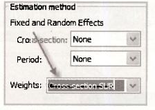
The coefficient estimates obtained in the previous section were obtained under the assumption that σ_GE = σ²_WE, and that the errors for the Westinghouse and General Electric equations, in the same year, are uncorrelated, cov(e_GE, e_WE) = 0. Seemingly unrelated regression estimates are obtained under the assumptions σ²_GE # σ²_WE and cov(e_GE ,e_WE,) # 0 . To obtain them we proceed exactly as we did in the previous section, with one slight modification. Can you remember the steps? Set up a pool object. Give it a name. This time we will call it SUR. Fill in the cross-section identifiers. Click Estimate. Fill in the Dependent variable and Cross-section specific coefficients boxes as before. The new thing that you need to do this time is to select Cross­section SUR from the drop-down Weights menu in the Estimation method box.

The results appear below. Compare them with Table 15.3 on page 388 of the text. The following points are worth noting.

1. In the output the coefficients are ordered according to variable. In Table 15.3 they are ordered according to equation.
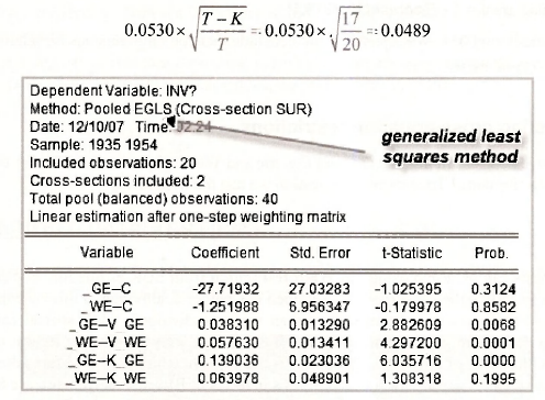
2. EViews calls the estimation method Pooled EGLS (estimated generalized least squares). The SUR estimator is a particular kind of generalized least squares estimator.
3. Although the coefficient estimates are identical to those in Table 15.3, the standard errors are not. The difference arises because EViews uses T as the divisor when estimating the error variances and covariance, whereas the degrees of freedom corrected divisor T -K was used for the results in Table 15.3. Both are popular. To reconcile the two, consider the last standard error reported from both places and note that

1.6. Testing contemporaneous correlation

In the context of the two-equation SUR model, a test for contemporaneous correlation is a test of H₀: cov(e_GE,e_WE ) = 0. The relevant test statistic, described on page 389 of the text, is LM = T x r²_GE.WE where r²_GE.WE is the squared correlation between the least squares residuals from the two equations. To get this correlation return to the pool object LS EQNS (we want least squares residuals not SUR residuals), open it, and select View/Residuals/Correlation Matrix.

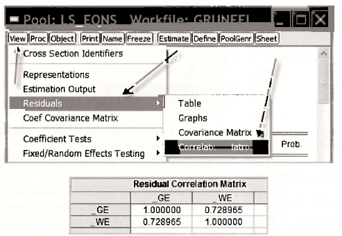
From the resulting matrix, we have r²_GE.WE = (0.728965)² = 0.53139 , giving a test statistic value of LM = 20×0.53139 = 10.628. The command

scalar pval = 1 – @cchisq(10.6278,1)

yields a p-value of 0.0011. We reject H₀ and conclude that contemporaneous correlation between the equation errors exists.

1.7. Testing cross-equation restrictions

So far we have been assuming that General Electric and Westinghouse have different coefficients. Could they be the same? To answer this question we test the hypothesis

This hypothesis can be tested using the Wald test option from SUR estimation. For carrying out the test we can follow the same steps as described in Chapter 6, although in this case the formulas for the test statistics are more complicated than we have divulged. Also, special care must be exercised to make sure we are testing the coefficients that we want to test. Return to the SUR output. Note the order of the coefficients. This is the order in which EViews stores them in the C vector. Consequently, writing the null hypothesis in terms of EViews coefficients, we have

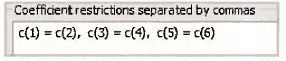
H₀: C(1)=C(2), C(3)=C(4), C(5)=C(6)

Select View/Coefficient TestsAVald – Coefficient Restrictions. Enter the following restrictions in the Wald test box.

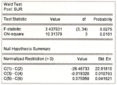
In the lower part of the output, the normalized restrictions are P_1.GE – P_1.WE = 0, P_2.GE – P_2.WE = 0  and P_{3 G£} -P₃._TO =0. Estimates of the left hand sides of the restrictions and their standard errors appear in the columns Value and Std. Err. The F- and y²-values for the test are given in the upper part of the output, along with their corresponding ^-values. The hypothesis of equal coefficients is rejected.

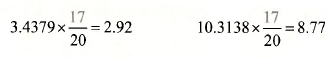
There is a discrepancy between the values in the text on pages 390-1 and those in the above output. Those in the text are F = 2.92 and x² = 8.77. The difference is again attributable to the treatment of a degrees of freedom correction when estimating the error variances and covariance. To convert the EViews values to the text values, we multiply by (17/20).

2. GRUNFELD DATA: TEN FIRMS

A more complete set of the Grunfeld data comprising T = 20 observations on A = 10 firms can be found in the workft\e grunfeld.wfl. The contents of this workfile are displayed below.

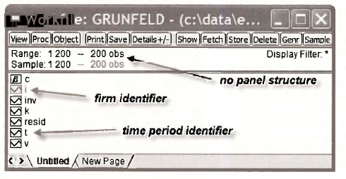
This file contains the familiar series INV, V and K and two new series I and T. The series I identifies observations for the i-th firm, i = 1,2,…, 10 . The series T identifies observations for the t-th time period, t = 1,2,…,20. The Range and Sample are both simply set at 1 200 without recognition of the panel structure of the data. So that EViews is fully informed, we begin this section by specifying the panel structure.

2.1. Structuring the workfile

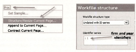
Go to Proc/Structure/Resize Current Page. A Workfile structure dialog box appears. There are various options that we could choose from the drop-down menu Workfile structure type. Since we have the identifying series / and T in the workfile, we choose undated with ID series and insert the names of these series in the Identifier series box.

When you return to the workfile, you will see extra information under Range that says Dim(10,20). In other words, the panel dimension is (10×20). EViews has figured out this dimension by checking the values in I and T.

2.2. Fixed effects using dummy variables

Table 15.4 on page 392 of the text presents estimates of the investment functions for the 10 firms assuming (1) all firms have the same coefficients on V and K, (2) each firm has a different intercept, (3) the error variances are the same for all firms, and (4) there is no contemporaneous correlation between errors of different firms. Taken together, these assumptions comprise those of a standard fixed effects model. The different intercept terms are known as fixed effects. The fixed effects model can be estimated in one of two ways. Dummy variables can be included for each of the firms and the constant omitted. In this case the coefficients of the dummy variables are the intercepts (fixed effects). Alternatively, the data can be expressed in terms of deviations from firm means and estimated without any intercepts, as described on page 394 of the text. We will first estimate the model by including dummy variables. Later we consider EViews automatic fixed effects option, and relate it back to our results for the dummy variable specification. We do not explicitly consider estimation using data expressed as deviations from firm means, although that is undoubtedly the approach taken by EViews automatic command.

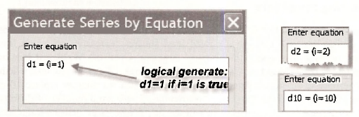
We generate the dummy variable series by using a sequence of logical generate commands. For example, the command

series d1 = (i=1)

generates a series D1 that is equal to one when (i=1) is true and equal to zero when (i=1) is false. Ten such commands are needed, one for each dummy variable.

To estimate the model, proceed to the Equation specification in the usual way. Enter the dependent variable INV, followed by each of the dummy variables, V and K. You will have noticed the Panel options tab at the top of the Equation estimation window. It is not needed. You might be tempted to select fixed effects. That would be wrong. Including the dummy variables means the fixed effects are already included. If you try to do it twice, EViews will get upset and send you a nasty singular matrix message.

Compare the above output with that in Table 15.4 of the text. Note the way EViews describes the panel structure in the top portion of the output.

2.3. Testing the effects

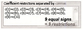
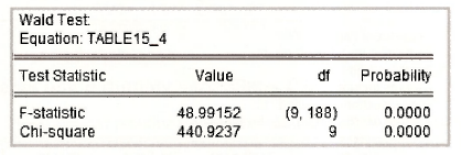
A test likely to be of interest is one that checks whether the intercepts for all Firms could be identical. If they are, one can use a pooled least squares regression estimated from the 200 observations without any regard for the panel structure. Open the Wald test box by going to View/Coefficient Tests/Wald – Coefficient Restrictions. We want to test whether the 10 intercept coefficients are equal. Another way of putting it is we want to replace 10 coefficients with one coefficient. To do so involves 9 restrictions. There are a number of different ways of writing these restrictions. One way appears in the box below. Note that the intercepts represent the first 10 coefficients and so they will be numbered C(l), C(2), …, C(10). Another alternative is to set C(l) = C(2), C(l) = C(3), …, C(l) = C(10). You will be able to think of other ways.

The upper panel of the test outcome appears below. Notice that the F-value is the same as that on page 393 of the text, obtained using restricted and unrestricted sums of squared errors. The relationship between the two test values is x² =9xF , with 9 being the degrees of freedom for the x² -test and the numerator degrees of freedom for the F-test. With p-values of 0.0000, both tests clearly reject the null hypothesis of equal intercepts.

2.4. Pooled least squares

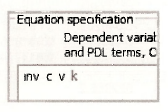
The pooled least squares estimates that make no special assumptions to accommodate the panel structure are given in Table 15.7 on page 395 of the text. No special commands are required to produce these estimates. Following the usual steps, leads to the Equation specification and results that appear below.

2.5. The fixed effects estimator

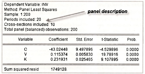
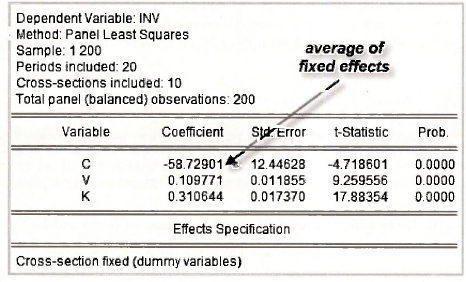
Now consider EViews automatic command for estimating a Fixed effects (dummy variable) model. You Fill in the same Equation specification as you did for the pooled least squares estimator in the previous section, but this time you need to click on the Panel options tab and choose Fixed for the Cross-section Effects specification.

The upper part of the output appears below. You should notice that the estimates for the coefficients of V and K are identical to those obtained when we explicitly included the dummy variables in Section 15.2.2. Also, if you took time to do the arithmetic, you would discover that the new intercept -58.729 is equal to the average of the dummy variable coefficients obtained earlier.

a. Retrieving the fixed effects

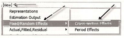
Sometimes the fixed effects (intercept estimates) are of special interest. They can be used to analyze the extent of firm heterogeneity and to examine any particular firms that may be of interest. For many examples the number of fixed effects is enormous and so rather than print them on the output, Eviews puts them in a special spreadsheet. To locate this spreadsheet go to View/Fixed/Random Effects/Cross-section Effects.

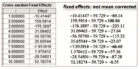
The spreadsheet for the fixed effects for each of the 10 firms is given in the left-hand side of the panel below. A comparison with the dummy variable coefficients from Table 15.4 reveals that they are not the same. The difference is that EViews has expressed them in terms of deviations form the mean of -58.729 that was reported on the output. To get the original fixed effects you add the mean as is done on the right-hand side of the below panel.

b. Testing the fixed effects

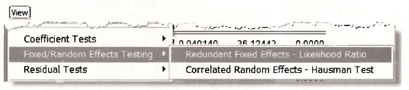
Can we use the fixed effects output to test for equality of the fixed effects (dummy variable coefficients) like we did earlier using the dummy variable specification? The answer is yes. Go to View/Fixed/Random Effects Testing/Redundant Fixed Effects – Likelihood Ratio.

Two versions of the likelihood ratio test appear in the output, an E-test and a x² -test. The E-test is identical to the one we considered earlier, and gives the same test results. The x²-test has a different origin, and so leads to a different test value. The details are beyond the level of our current description, but you can get a feel for where it comes from by checking equation (C.25) on page 537 of the text.

3. THE NLS PANEL DATA

The data in the file nls_panel.wfl is from the National Longitudinal Surveys conducted by the U.S. Department of Labor. This file is a large one that, in its current form, cannot be saved by the Student Version of EViews. We can nevertheless use the Student Version to analyze the data. After you have finished estimation, if you wish to save your results, you will need to reduce the range of the workfile structure and delete some of the series until the file is small enough to be saved by EViews Student Version. When saving it, name it differently, say nls results.wfl. You will then have two files, the original one with the data and another one with your results. This is an inconvenient state of affairs, but not an impossible scenario. The other alternative is to pay more for convenience and buy the EViews full version.

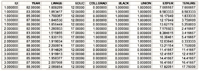
Opening the file reveals 3580 observations with a panel structure comprising 5 time series observations (1982, 1983, 1987, 1988) on 716 individuals.

We can check the data against that in Table 15.8 by collecting those variables into a group and examining the following spreadsheet.

3.1. Fixed effects estimation

The first model estimated using the NLS panel is a fixed effects model with In (WAGE) as the dependent variable and explanatory variables EXPER, EXPER2, TENURE, TENURE2, SOUTH and UNION. It is also suggested that we try a fixed effects model with EDUC and BLACK included to see what happens. Estimation should fail because EDUC and BLACK are constant over time for each individual. Their effects will be captured by the individual fixed effects. The Equation specification and Effects specification (selected form the Panel options) for this model are

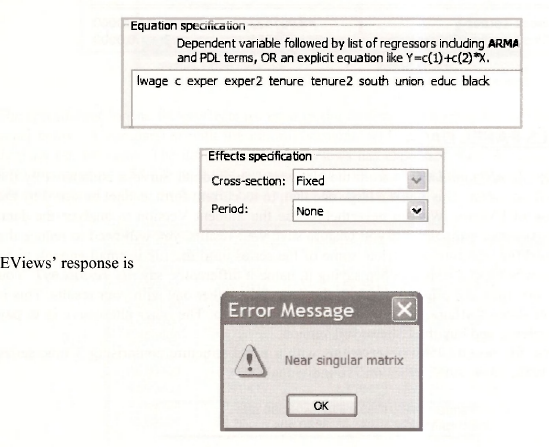
This is a message that you will see if you try to estimate a model with perfect collinearity among the explanatory variables. In fact, EViews is being kind. The relevant matrix is singular not just “nearly” singular. We have not been specific about the matrix to which EViews refers. At this stage of your career is is sufficient to know that the singularity is caused by collinear explanatory variables.

After dropping the offending variables EDUC and BLACK, the specification is

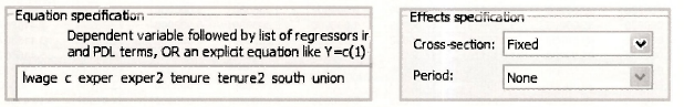
The output follows. Note the correspondence with the results in Table 15.9 on page 397 of the text.

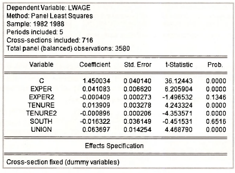
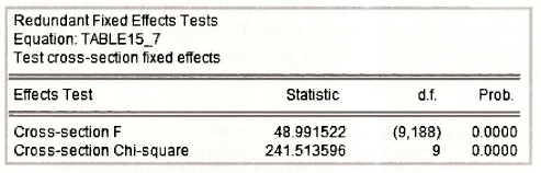
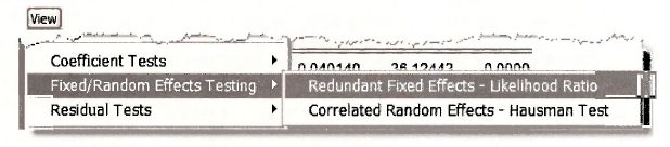
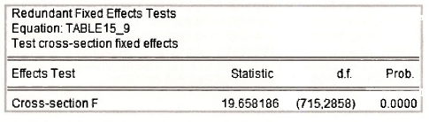
To test for the presence of individual differences we test the equality of the fixed effects as described in Section 15.2.5b. Go to View/Fixed/Random Effects Testing/Redundant Fixed Effects – Likelihood Ratio.

The resulting test details confirm the F-value of 19.66 reported on page 398 of the text.

3.2. Random effects estimation

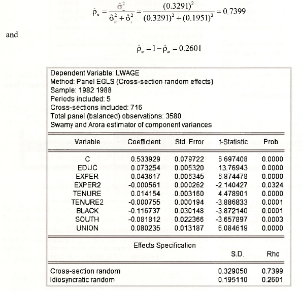
Individual effects that were modeled by fixed coefficients in the fixed effects model are treated as random draws from a larger population in the random effects model. For estimation purposes they become part of the error term. Also, estimation of the random effects model takes into account variation between individuals as well as variation within individuals. For our data set, this means it is possible to include EDUC and BLACK in the model. Doing so leads to the following Equation and effects specifications.

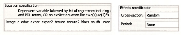
The output that follows yields the results in Table 15.10 on page 402 of the text. In the lower part of the output, cross section random refers to the estimate o_a =0.3291 and idiosyncratic random refers to the estimate o_e = 0.1951. The values in the column rho are the proportions of total error variance attributable to each of the components. Thus,

3.3. The Hausman test

The ability of the random effects model to take into account variation between individuals as well as variation within individuals makes it an attractive alternative to fixed effects estimation. However, for the random effects estimator to be unbiased in large samples the effects must be uncorrelated with the explanatory variables, an assumption that is often unrealistic. This assumption can be tested using a Hausman test. The Hausman test is a test of the significance of the difference between the fixed effects estimates and the random effects estimates. Correlation between the random effects and the explanatory variables will cause these estimates to diverge; their difference will be significant. If the difference is not significant, there is no evidence of the offending correlation. The differences between the two sets of estimates can be tested separately using t-tests,, or as a block using a x²-test.

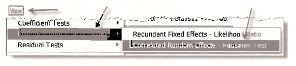
You can ask EViews to perform a Hausman test by opening the random-effects estimated equation and going to View/Fixed/Random Effects Testing/Correlated Random Effects – Hausman Test.

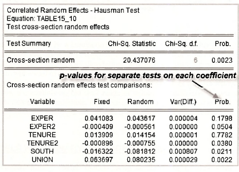
For the wage equation we get the following results. The value of the -statistic for testing differences between all coefficients is x² = 20.437 . Its corresponding p-\alue of 0.0023 suggests the null hypothesis of no correlation between the explanatory variables and the random effects should be rejected. The p-values for separate tests on the differences between each pair of coefficients are given in the column Prob. The results here are mixed. At a 5% significance level, the null hypothesis is rejected for TENURE2, SOUTH and UNION, but not for EXPER, EXPER1 and TENURE. These results are slightly different to those reported on pages 205-206 of the text, but not enough to suggest anything is wrong. Differences may have occurred because of different covariance matrix estimators.

Source: Griffiths William E., Hill R. Carter, Lim Mark Andrew (2008), Using EViews for Principles of Econometrics, John Wiley & Sons; 3rd Edition.