Interval Estimation and Hypothesis Testing by using EViews

1. INTERVAL ESTIMATION

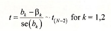
For the regression model y = β₁ +β₂x + e, and under assumptions SR1-SR6, the important result that we use in this chapter is given in equation (3.3) of POE.

            ’

Using this result we can show that the interval b_k ± t_cse(b_k) has probability 1-a of containing the true but unknown parameter p*, where the “critical value” t_c from a /-distribution such that P(t>t_c) = P(t<-t_c) = a/2

To construct interval estimates we will use EViews’ stored regression results. We will also make use of EViews built in statistical functions. For each distribution (see Function reference in EViews Help) four statistical functions are provided. The two we will make use of are the cumulative distribution (CDF) and the quantile (Inverse CDF) functions.

The for the /-distribution the CDF is given by the function @ctdist(x,v). This function returns the probability that a /-random variable with v degrees of freedom falls to the left of x. That is,

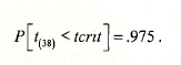
The quantile function @qtdist(p,v) computes the critical value of a /-random variable with v degrees of freedom such that probability p falls to the left of it. For example, if we specify tc=@qtdist(.975,38), then

To construct the interval estimates we require the least squares estimates bk and their standard errors se(bk). After each regression model is estimated the coefficients and standard errors are saved in the arrays @coefs and @stderrs. However they are saved only until the next regression is run, at which time they are replaced. If you have named the regression results, as we have (FOOD_EQ) then the coefficients are saved as well, with the names food_eq.@coefs and food_eq.@stderrs, respectively.

1.1. Constructing the interval estimate

Since we have estimated only one regression we can use the simple form for the saved results. Thus @coefs(2) = b2 and @stderrs(2) = se(b2). To generate the 95% confidence interval [b₂ – t_cse{b₂), b₂ + t_cse(b₂)\ enter the following commands in the EViews command window, pressing the <Enter> key after each:

scalar tc = @qtdist(.975,38)

scalar b2 = @coefs(2)

scalar seb2 = @stderrs(2)

scalar b2_lb = b2 – tc*seb2

scalar b2_ub = b2 + tc*seb2

These scalar values show up in the workfile with the symbol #. For example, the value of the lower bound of the interval estimate is

1.2. Using a coefficient vector

While the above approach works perfectly fine, it may be nicer for report writing to store the interval estimates in an array and construct a table. On the main EViews Menu select Objects/New Object

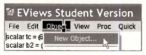
We will create a Matrix-Vector-Coef named INT EST

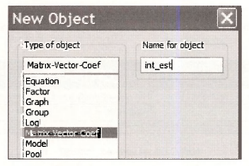
It will be a coefficient vector that has 2 rows and 1 column

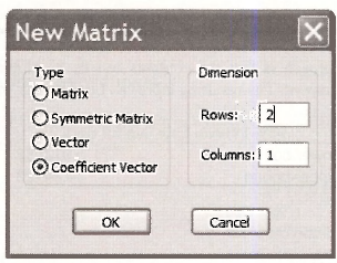
Click OK, and the empty array appears. Instead of all that pointing and clicking, you can simply enter on the command line

coef(2) int_est

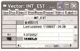
Now, enter the commands

int_est(1) = @coefs(2) – @qtdist(.975,38)*@stderrs(2)

int_est(2) = @coefs(2) + @qtdist(.975,38)*@stderrs(2)

Here we have used the EViews saved results directly rather than create scalars for each elements. The vector we created is

Click on Freeze and then Name. We chose the name B2 INTERVAL ESTIMATE and it looks like this:

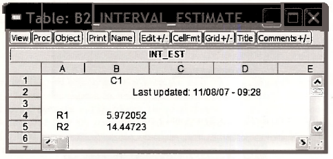
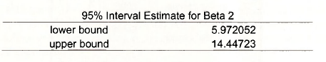
The advantage of this approach is that the contents can be highlighted, copied (Ctrl+C) and pasted (Ctrl+V) into a document. The resulting table can be edited as you like

2. RIGHT-TAIL TESTS

2.1. Test of significance

To test the null hypothesis that (3₂ = 0 against the alternative that it is positive (> 0), as described in Chapter 3.4.1a of POE, requires us to find the critical value, construct the /-statistic, and determine the /7-value.

• If we choose the a = .05 level of significance, then the critical value is the 95^th percentile of the /(3g) distribution.
• The /- statistic is the ratio of the estimate bi over its standard error, se(b₂).
• The /7-value is the area to the right of the calculated /-statistic (since it is a right-tail test). This value is one minus the cumulative probability to the left of the /-statistic.

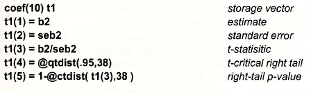
The simplest set of commands is (do not type the comments in italic font)

scalar tc95 = @qtdist(.95,38)                           t-critical right tail

scalar tstat = b2/seb2                                       t-statistic

scalar pval = 1 – @ctdist(tstat,38)                    right-tail p-value

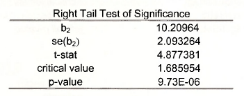
Alternatively, use the vector approach outlined in the previous section

Use the results of this vector to construct a table, such as

2.2. Test of an economic hypothesis

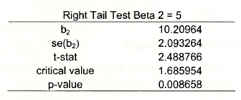
To test the null hypothesis that β₂ < 5 against tl alternative β₂ > 5 the same steps are executed, except for the construction of the t-statistic.

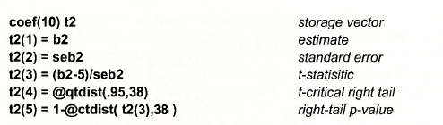
Yielding

3. LEFT-TAIL TESTS

3.1. Test of significance

To test the null hypothesis that β₂ > 0 against the alternative that it is negative (< 0) requires us to find the critical value, construct the t-statistic, and determine the p-value.

• If we choose the a = .05 level of significance, then the critical value is the 5^th percentile of the t(38) distribution.
• The t- statistic is the ratio of the estimate b₂ over its standard error, se(b₂).
• The p-value is the area to the left of the calculated /-statistic (since it is a left-tail test). This value is given by the cumulative probability to the left of the t-statistic.

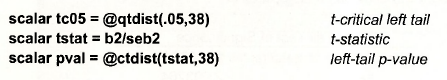
The simplest set of commands is (do not type the comments in italic font)

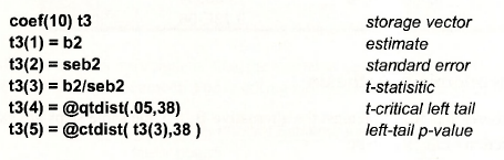
Alternatively

Yielding

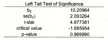
Note that we fail to reject the null hypothesis in this case, as expected.

3.2. Test of an economic hypothesis

To test the null hypothesis that β₂ >12 against the alternative that β₂ < 12, we use the same steps as above, except for the construction of the t-statistic.

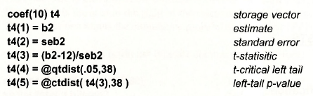
Yielding,

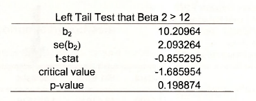
The t-statistic value -.85 does not fall in the rejection region, and the p-value is about .20, thus we fail to reject this null hypothesis.

4. TWO-TAIL TESTS

4.1. Test of significance

The two tail test of the null hypothesis that β₂ = 0 against the alternative that β₂ # 0 we require the same test elements

• If we choose the a = .05 level of significance, then the right-tail critical value is the 97.5- percentile of the f₍38) distribution and the left tail critical value is the 2.5-percentile.
• The t- statistic is the ratio of the estimate bi over its standard error, se(£>->).
• The p-value is the area to the left of minus the absolute value of the calculated t-statistic plus the area to the right of the absolute value of the calculated test statistic (since it is a two-tail test). This value is given by the cumulative probability to the left of the – |t-statistic| and l – the cumulative probability to the right of |t-statistic|.

The two tail p-value is

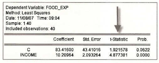
The test is carried out by EViews each time a regression model is estimated. If we examine FOOD_EQ, in the column labeled t-statistic is the ratio of the Coefficient to Std. Error. The column labeled Prob. contains the two-tail p-value for the test of significance. Note that the very small p-value is rounded to zero (to 4 places). For practical purposes this is enough since levels of significance below .001 are hardly ever used.

To use the coefficient vector approach

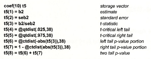
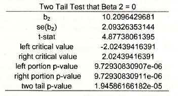
The result is as follows. Here we have copied the results from EViews at the highest precision to show that the p-value works out to be the same as reported above.

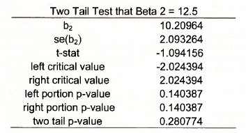
4.2. Test of an economic hypothesis

To test the null hypothesis that β₂ = 12.5 against the alternative β₂ # 12.5 the steps are the same as those above, except for the construction of the t-statistic.

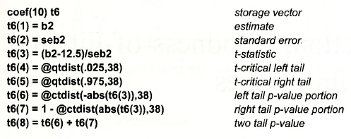
Which yields

Source: Griffiths William E., Hill R. Carter, Lim Mark Andrew (2008), Using EViews for Principles of Econometrics, John Wiley & Sons; 3rd Edition.