The Simple Linear Regression Model by using EViews

In this chapter we introduce the simple linear regression model and estimate a model of weekly food expenditure. We also demonstrate the plotting capabilities of EViews and show how to use the software to calculate the income elasticity of food expenditure, and to predict food expenditure from our regression results.

1. OPEN THE WORKFILE

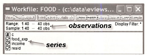
The data for the food expenditure example are contained in the workfile food.wfl. Locate this file and open it by selecting File/Open/EViews Workfile

The initial workfile contains two variables INCOME, which is weekly household income, and FOOD EXP, which is household weekly household food expenditure. See the definition file foocLdef for the variable definitions.

1.1. Examine the data

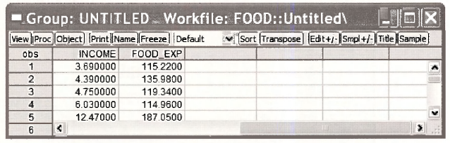
When ever opening a new workfile it is prudent to examine the data. Select INCOME by clicking it, and then while holding the Ctrl-key select FOOD EXP.

Double-click in the blue area and select Open Group. The data appear in a spreadsheet format, with INCOME first since it was selected first.

1.2. Checking summary statistics

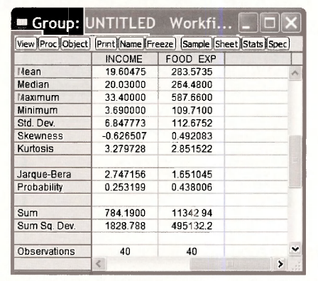
In the definition file food.def we find variable definitions and summary statistics.

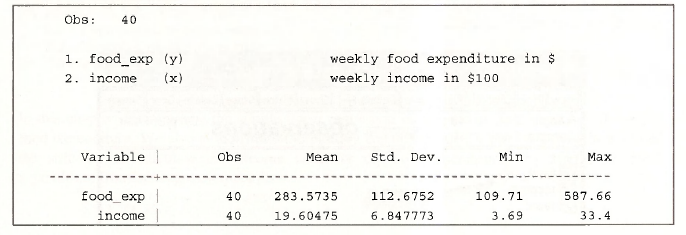
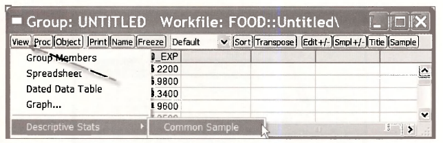
To verify that the workfile we are using agrees, select View/Descriptive Stats/Common Sample.

The resulting summary statistics agree with the information in the food.de/which assures us that we have the correct data.

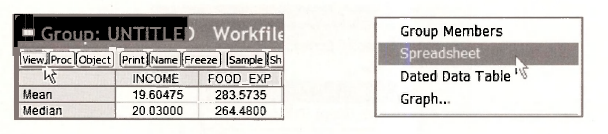
To return to the spreadsheet view, select View/Spreadsheet

1.3. Saving a group

It is often useful to save a particular group of variables that are in a spreadsheet. From within the Group screen select Name and then assign an Object Name. Click OK.

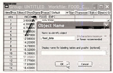
The new object in the workfile is a Group named FOOD DATA.

2. PLOTTING THE FOOD EXPENDITURE DATA

With any software there are several ways to accomplish the same task. We will make use of EViews “drop-down menus” until the basic commands become familiar. Click on Quick/Graph

In the dialog box type the names of the variables with the x-axis variable coming first!

In the Graph Options box select Scatter from among the Basic graphs.

A plot appears, to which we can add labels and a title.

2.1. Enhancing the graph

While the basic graph is fine, for a written paper or report you it can be improved by

• adding a title
• changing vertical axis scale

These tasks are easily accomplished. To add a title, click on AddText on the Graph menu.

In the resulting dialog box you will be able to add a title, specify the location of the title, and use some stylistic features.

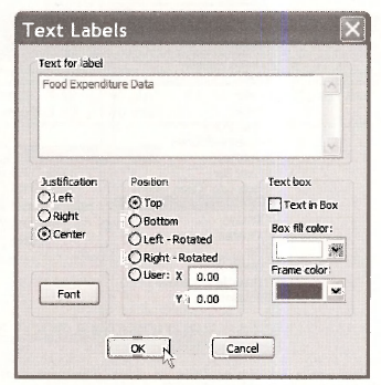
To have the title centered at the top click the appropriate options and type in the title. Click OK.
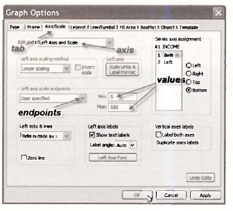
To alter the vertical axis so that it begins at zero, click on Options on the Graph Menu

Click on the Axes/Scale tab, select the Left Axis and Scale option in the drop down box. Choose User specified in the Left axis scale method. Enter 0 and 600 as the Min and Max values. Click OK.

To change the “empty circles” used in the graph to “filled circles”, again choose Options, but select the Line/Symbol tab.

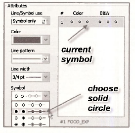
Click on Symbol pattern and choose the style you want. Note that other options are available. Click OK. The resulting graph is now

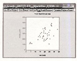
Explore the other tabs on the Options menu to see all the features.

2.2. Saving the graph in the workfile

To save the graph, so that it remains in the workfile, click on Name, then enter a name. Note that separate words are not allowed, but separating words with an underscore is an alternative.

In the workfile, you will find an icon representing the graph just created

2.3. Copying the graph to a document

As is usual with Windows based applications, we can copy by clicking somewhere inside the graph, to select it, then Ctrl+C. Or in the main window click on Edit/Copy

The dialog box that shows up allows you to choose the file format. Switch to your word processor and simply paste the graph (Ctrl+V) into the document.

To save the graph to disk, select the Object button on the Graph menu.

Select View Options/Save graph to disk. In the resulting dialog box you have several file types to choose from, and you can select a name for the graph image.

2.4. Saving a workfile

You may wish to save your workfile at this point. If you select the Save button on the workfile menu the workfile will be saved under its current name food.w/1. It might be better to save this file under a new name, so that the original workfile remains untouched. Select File/Save As on the EViews menu and select a simple but informative name.

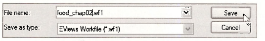
We will name it food_chap02.wfl

3. ESTIMATING A SIMPLE REGRESSION

To estimate the parameters b\ and b-> of the food expenditure equation, we select Quick/Estimate Equation from the EViews menu.

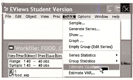
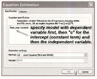
In the Equation Specification dialog box, type the dependent variable FOOD EXP (the y variable) First, C (which is EViews notation for the intercept term, or constant), and then the independent variable INCOME (the x variable). Note in the Estimation settings window, the Method is Least Squares and the Sample is 1 40. Click OK.

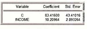
The estimated regression output appears. EViews produces an equation object in its default Stats view. We can name the equation object to save it permanently in our workfile by clicking on Name in the equation’s toolbar. We have named this equation FOOD_EQ.

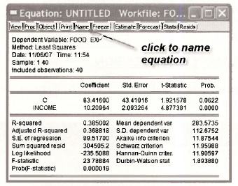
Note the estimated coefficient bi, the intercept in our food expenditure model is recorded as the coefficient on the variable C in EViews. C is the EViews term for the constant in a regression model. Note that we cannot name any of our variables C since this term is reserved exclusively for the constant or “intercept” in a regression model. Our EViews output shows b\ — 83.4160. The estimated value of the slope coefficient on the variable weekly income (X) is b₂ – 10.2096, as reported in POE, Chapter 2.3.2. The interpretation of b₂ is: for every $100 increase in weekly income we estimate that there is about a $10.21 increase in weekly food expenditure, holding all other factors constant.

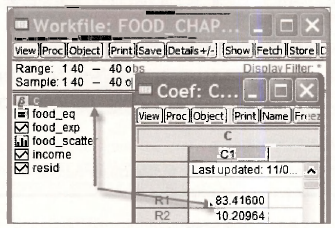
In the workfile window, double click on the vector object C. It always contains the estimated coefficients from the most recent regression.

The vector RESID always contains the least squares residuals from the most recent regression. We will return to this shortly.

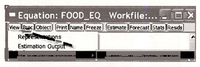
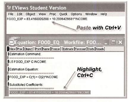
3.1. Viewing equation representations

One EViews button that we will use often is the View button in a regression window

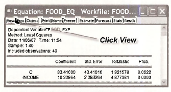
On the drop down menu list click Representations

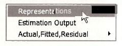
The resulting display shows three things:

• The Estimation Command is what can be typed into the command line to obtain the equation results.
• The Estimation Equation that shows the coefficients and how they are linked to the variables on the equation’s right side: C( 1) is the intercept and C(2) is the slope
• The Substituted Coefficients displays the fitted regression line.

To return to the regression window click Stats.

3.2. Computing the income elasticity

As shown in equation (2.9) of POE the income elasticity is defined to be

which is then implemented by replacing unknowns by estimated quantities,

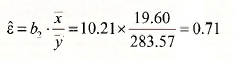
We can use EViews as a “calculator” by simply typing into the command line

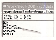
then pressing Enter. The word scalar means that the result is a single number. An icon appears in the workfile,

Double-click in the shaded area, and in the lower left comer of the EViews screen you will find the result

While this gives the answer, there is something to be said for using the power of EViews to simplify the calculations. EViews saves the estimates from the most recent regression in the workfde. They are obtained by double clicking the “β” icon

These coefficients can be accessed from the array @coefs. Also, EViews has functions to compute many quantities. The arithmetic mean is computed using the function @mean. Thus the elasticity can also be obtained by entering into the command line

scalar elast2 = @coefs(2)*@mean(income)/@mean(food_exp)

The result is slightly different than the first computation because in the first we used “rounded off’ values of the sample means.

Because the array @coefs is not permanent, you may want to save the slope estimate as a separate quantity by entering the commands

scalar b2 = @coefs(2)

scalar elast3 = b2*@mean(income)/@mean(food_exp)

However, the coefficient array can always be retrieved if the food equation has been saved and named. Recall that we did save it with the name FOOD_EQ. By saving the equation we also save the coefficients, which can by retrieved from the array FOOD_EQ.@coefs.

scalar elas = food_eq.@coefs(2)*@mean(income)/@mean(food_exp)

We have some surplus icons in our workfile now. Keep B2 and ELAS. To clean out the other elasticties, highlight (hold down Ctrl and click each), right-click in the blue area, and select Delete. Save the workfile.

4. PLOTTING A SIMPLE REGRESSION

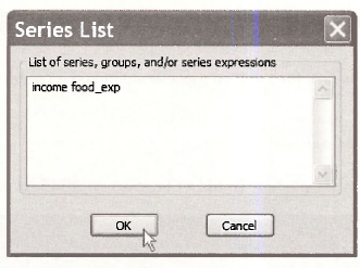
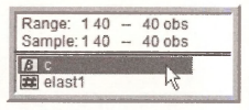
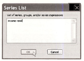
Select Quick/Graph from the EViews menu. In the Series List dialog box enter INCOMEand FOOD EXP.

On the Type tab select Scatter

In the Details section, using the Fit lines drop down menu, select Regression Line.

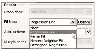
Edit the scale of the vertical axis, choose solid circles for data points, and add a title as shown in Section 2.2.1. Click inside the graph, enter Ctrl+C, OK, and then paste into a document using Ctrl+V. The graph should look like this.

Return to EViews and in the Graph window select the Name button and assign a name to this object, such as FITTED LINE.

5. PLOTTING THE LEAST SQUARES RESIDUALS

The least squares residuals are defined as

As you will discover these residuals are important for many purposes. To view the residuals open the saved regression results in FOOD_EQ by double clicking the icon.

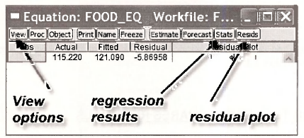
5.1. Using View options

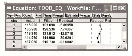
Within the equation FOOD_EQ window, click on View then Actual, Fitted, Residual. There you can select to view a table or several graphs.

If you select Actual, Fitted, Residual Table you will see the values of the dependent variable y, the predicted (fitted) value of y, given by y = b, + b₂x and the least squares residuals, along with a plot.

5.2. Using Resids plot

Within the object FOOD_EQ you can navigate by selecting buttons. Select Resids.

The result is a plot showing the least squares residuals (lower graph) along with the actual data (FOOD EXP) and the fitted values. When using this plot note that the horizontal axis is the observation number and not INCOME. In this workfile the data happen to be sorted by income, but note that the fitted values are not a straight line. When examining residual plots, a lack of pattern is consistent with the assumptions of the simple regression model.

5.3. Using Quick/Graph

To create a graph of the residuals against income we can use the fact the EViews saves the residuals from the most recent regression in the series labeled RESID. Click on Quick/Graph. In the dialog box enter INCOME (x-axis comes first) and RESID.

Choose the Scatter plot. The resulting plot shows how the residuals relate to the values of income.

Save this plot by selecting Name and assigning RESIDUAL_PLOT.

5.4. Saving the residuals

To save these residuals for later use, we must Generate a new variable (series). In the workfile screen click Genr on the menu.

[Genr|

In the resulting dialog box create a new variable called EHAT that contains the residuals

 

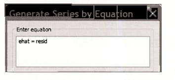
Click OK. Alternatively, simply type into the command line

series ehat = resid

6. ESTIMATING THE VARIANCE OF THE ERROR TERM

The estimator for σ², the variance of the error term is

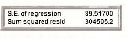
where Sum squared resid is the EViews name for the sum of squared residuals. The square root of the estimated error variance is called the Standard Error of the Regression by EViews,

Open the regression equation we have saved as FOOD_EQ. Below the estimation results you will find the Standard Error of the Regression and the sum of squared least squares residuals.

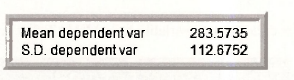
Also reported are the sample mean of the y values (Mean dependent variable)

The sample standard deviation of the y values (S.D. dependent var) is

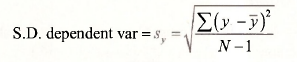
These are

7. COEFFICIENT STANDARD ERRORS

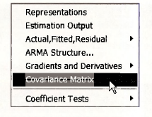
The estimated error variance is used to construct the estimates of the variances and covariances of the least squares estimators as shown in POE equations (2.20)-(2.22). These estimated variances can be viewed from the FOOD_EQ regression by clicking on View/Covariance Matrix

The elements are arrayed as

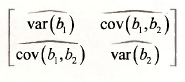
In EViews they appear as

The highlighted value is the estimated variance of b₂. If we take the square roots of the estimated variances, we obtain the standard errors of the estimates. In the regression output these standard errors are denoted Std. Error and are found right next to the estimated coefficients.

8. PREDICTION USING EVIEWS

There are several ways to create forecasts in EViews, and we will illustrate two of them.

8.1. Using direct calculation

Open the food equation FOOD_EQ. Click on View/Representations. Select the text of the equation listed under Substituted Coefficients. We can choose Edit/Copy from the EViews menubar, or we can simply use the keyboard shortcut Ctrl+C to copy the equation representation to the clipboard. Finally, we can paste the equation into the command line.

To obtain the predicted food expenditure for a household with weekly income of $2000, edit the command line to read

scalar FOOD_EXP_HAT = 83.4160020208 + 10.2096429681*20

Press Enter. The resulting scalar value is

which is correct to more decimals than the value 287.61 we report in Chapter 2.3.3b.

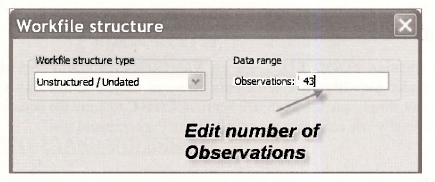
8.2. Forecasting

A more general, and flexible, procedure uses the power of EViews. In order to predict we must enter additional x observations at which we want predictions. In the main workfile window, double-click Range. This workfile has an Unstructured/Undated structure. Change the number of observations to 43.

Click OK. EViews will check with you to confirm your action.

Next, double-click on INCOME in the main workfile to open the series, and click the Edit+/- button in the series window, which puts EViews in edit mode.

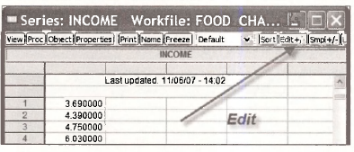
Scroll to the bottom and you see NA in the cells for observations 41-43. Click the cell for observation 41 and enter 20. Enter 25 and 30 in cells 42 and 43, respectively. When you are done, click the Edit+/- button again to turn off the edit mode.

Now we have 3 extra INCOME observations that do not have FOOD EXP observations. When we do a regression EViews will toss out the missing observations, but it will use the extra INCOME values when creating a forecast.

To forecast, first re-estimate the model with the original data. This step is not actually necessary, but we want to illustrate a point. Click on Quick/Estimate Equation. Enter the equation. Note in the dialog box that the Sample is 1 to 43.

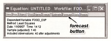
The estimation results are the same, and EViews tells us that the Included observations are 40 after adjustments. The 3 observations with not values for FOOD EXP were discarded.

To forecast with the estimated model, click on the Forecast button in the equation window.

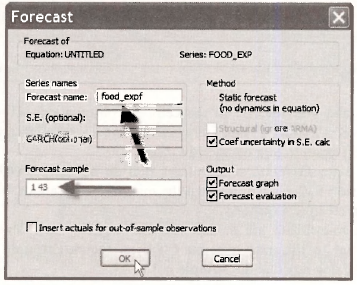
The Forecast dialog box appears. EViews automatically assigns the name FOOD_EXPF to the forecast series, so if you want a different name enter it. The Forecast sample is 1 to 43. Predictions will be constructed for the 40 samples values and for the 3 new values of INCOME. For now, ignore the other options. Click OK.

A graph appears showing the fitted line for observations 41-43 along with lines labeled ±2 S.E. We will discuss these later. To see the fitted values themselves, in the workfile window, double click on the series named FOOD EXPF and scroll to the bottom.

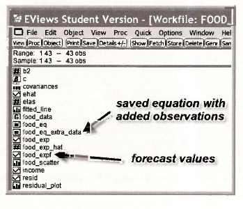
There you see the three forecast values corresponding to incomes 20, 25 and 30. The value in cell 41 is 287.6089, which is the same predicted value we obtained earlier in Chapter 2.3.3b.

While this approach is somewhat more laborious, by using it we can generate forecasts for many observations at once. More importantly, using EViews to forecast will make other options available to us that simple calculations will not.

Source: Griffiths William E., Hill R. Carter, Lim Mark Andrew (2008), Using EViews for Principles of Econometrics, John Wiley & Sons; 3rd Edition.