VEC and VAR Models by using EViews: An Introduction to Macroeconometrics

1. VEC AND VAR MODELS

A VAR model describes a system of equations in which each variable is a function of its own lag and the lag of the other variables in the system. A VEC model is a special form of the VAR for 1(1) variables which are cointegrated.

2. ESTIMATING A VEC MODEL

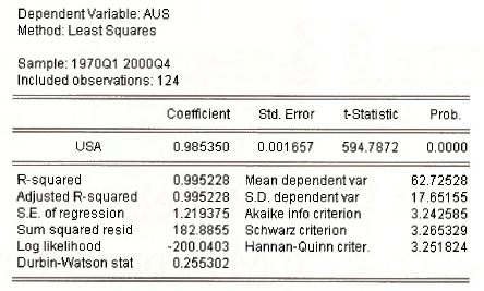
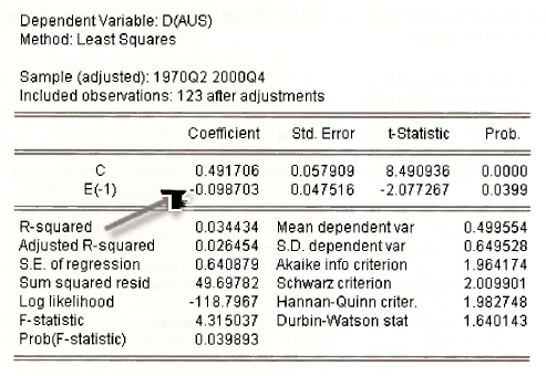
The results in the text were based on data contained in the EViews workfile gdp.wfl. The variables are AUS (real GDP for Australia) and USA (real GDP for US). To check whether the variables A US and USA are cointegrated or spuriously related, we need to test the regression residuals for stationarity. To do this, first estimate the following least squares equation.

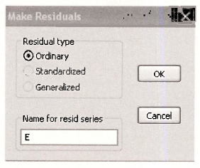
Next click Proc and select Make Residual Series from the drop-down menu to generate the residuals.

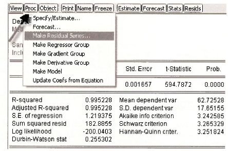
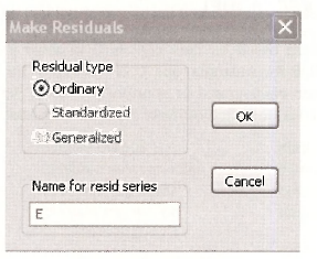
Following notation in the text, call the residual E.

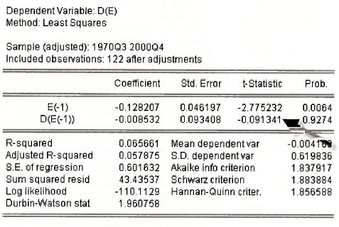
Next perform the unit root test by regressing the change of the residual d(e) on the lagged residual e(-1) as shown below.

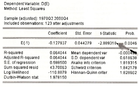
Since the calculated unit root test value (-2.889) is less than the critical value (-2.76, see Table 12.3), the null of no cointegration is rejected.

As an aside, extra lags of the dependent variable (for example d(e(-1)) were not introduced in the test equation above, as they were insignificant. See for example the case below.

The estimated error-correction equations are shown below. The error correction coefficients are the parameters of the lagged residual term, namely e(-1) above.

3. ESTIMATING A VAR MODEL

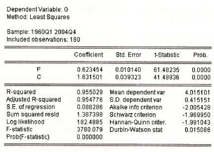
The results in the text were based on data contained in the EViews workfile growth.wfl. The variables are G (log of GDP) and P (log of the CPI). To check whether the variables are cointegrated or spuriously related, we need to test the regression residuals for stationarity. To do this, first estimate the following least squares equation.

Then, click on Proc and select Make Residual Series from the drop down menu.

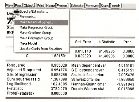
Following notation in the text, call the residuals E:

Next perform the unit root test by regressing the change of the residual d(e) on the lagged residual e(-1) as shown below.

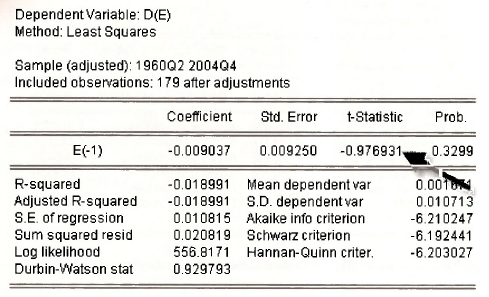
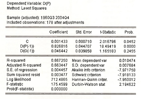
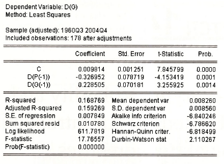
Since the calculated tau statistic (-0.977) is greater than the 5% critical value (-3.37, see Table 12.3), we accept the null of no cointegration. In other words, the variables are spuriously related. The estimated VAR equations are estimated by least squares as shown below.

4. IMPULSE RESPONSES AND VARIANCE DECOMPOSITION

In the text, we discuss the interpretation of impulse responses and variance decomposition for the special case where the shocks are uncorrelated. This is not usually the case, and EViews is set up for the more general cases when identification is an issue.

Source: Griffiths William E., Hill R. Carter, Lim Mark Andrew (2008), Using EViews for Principles of Econometrics, John Wiley & Sons; 3rd Edition.