Five Analytic Techniques in Case Study Research

None of the analytic techniques should be considered easy to use, and all will need much practice to be used powerfully. Your objective should be to start modestly, work thoroughly and introspectively, and build your own analytic repertoire over time. The reward will eventually emerge in the form of com­pelling case study analyses and, ultimately, compelling case studies.

1. Pattern Matching

For case study analysis, one of the most desirable techniques is to use a pattern-matching logic. Such a logic (Trochim, 1989) compares an empiri­cally based pattern with a predicted one (or with several alternative predic­tions). If the patterns coincide, the results can help a case study to strengthen its internal validity.

If the case study is an explanatory one, the patterns may be related to the dependent or the independent variables of the study (or both). If the case study is a descriptive one, pattern matching is still relevant, as long as the predicted pattern of specific variables is defined prior to data collection.

Nonequivalent dependent variables as a pattern. The dependent-variables pattern may be derived from one of the more potent quasi-experimental research designs, labeled a “nonequivalent, dependent variables design” (Cook & Campbell, 1979, p. 118). According to this design, an experiment or quasi-experiment may have multiple dependent variables—that is, a vari­ety of relevant outcomes. For instance, in quantitative health studies, some outcomes may have been predicted to be affected by a treatment, whereas other outcomes may have been predicted not to be affected (Rosenbaum, 2002, pp. 210-211). For these studies as well as a case study, the pattern matching occurs in the following manner: If, for each outcome, the initially predicted values have been found, and at the same time alternative “pat­terns” of predicted values (including those deriving from methodological artifacts, or “threats” to validity) have not been found, strong causal infer­ences can be made.

For example, consider a single case in which you are studying the effects of a newly decentralized office computer system. Your major proposition is that—because each peripheral piece of equipment can work independently of any server—a certain pattern of organizational changes and stresses will be produced. Among these changes and stresses, you specify the following, based on propositions derived from previous decentralization theory:

• employees will create new applications for the office system, and these applica­tions will be idiosyncratic to each employee;
• traditional supervisory links will be threatened, as management control over work tasks and the use of central sources of information will be diminished;
• organizational conflicts will increase, due to the need to coordinate resources and services across the decentralized units; but nevertheless,
• productivity will increase over the levels prior to the installation of the new system.

In this example, these four outcomes each represent different dependent vari­ables, and you would assess each with different measures. To this extent, you have a study that has specified nonequivalent dependent variables. You also have predicted an overall pattern of outcomes covering each of these variables. If the results are as predicted, you can draw a solid conclusion about the effects of decentralization. However, if the results fail to show the entire pattern as pre­dicted—that is, even if one variable does not behave as predicted—your initial proposition would have to be questioned (see BOX 26 for another example).

BOX 26

Pattern Matching on Each of Multiple Outcomes

Researchers and politicians alike recognize that U.S. military bases, located across the country, contribute significantly to a local economy’s housing, employment, and other markets. When such bases close, a corresponding belief is that the community will suffer in some catastrophic (both economic and social) manner.

To test the latter proposition, Bradshaw (1999) conducted a case study of a do- sure that had occurred in a modestly sized California community. He first identified a series of sectors (e.g., housing sales, civilian employment, unemployment, popula­tion turnover and stability, and retail markets) where catastrophic outcomes might have been feared, and he then collected data about each sector before and after the base closure. A pattern-matching procedure, examining the pre-post patterns of outcomes in every sector and also in comparison to other communities and statewide trends, showed that the outcomes were much less severe than antici­pated. Some sectors did not even show any decline. Bradshaw also presented evi­dence to explain the pattern of outcomes, thereby producing a compelling argument for his conclusions.

This first case could then be augmented by a second one, in which another new office system had been installed, but of a centralized nature—that is, the equipment at all of the individual workstations had been networked. Now you would predict a different pattern of outcomes, using the same four dependent variables enumerated above. And now, if the results show that the decentral­ized system (Case A) had actually produced the predicted pattern and that this first pattern was different from that predicted and produced by the centralized system (Case B), you would be able to draw an even stronger conclusion about the effects of decentralization. In this situation, you have made a theo­retical replication across cases. (In other situations, you might have sought a literal replication by identifying and studying two or more cases of decen­tralized systems.)

Finally, you might be aware of the existence of certain threats to the valid­ity of this logic (see Cook & Campbell, 1979, for a full list of these threats). For example, a new corporate executive might have assumed office in Case A, leaving room for a counterargument: that the apparent effects of decentraliza­tion were actually attributable to this executive’s appointment and not to the newly installed office system. To deal with this threat, you would have to iden­tify some subset of the initial dependent variables and show that the pattern would have been different (in Case A) if the corporate executive had been the actual reason for the effects. If you only had a single-case study, this type of procedure would be essential; you would be using the same data to rule out arguments based on a potential threat to validity. Given the existence of a sec­ond case, as in our hypothetical example, you also could show that the argu­ment about the corporate executive would not explain certain parts of the pattern found in Case B (in which the absence of the corporate executive should have been associated with certain opposing outcomes). In essence, your goal is to identify all reasonable threats to validity and to conduct repeated comparisons, showing how such threats cannot account for the dual patterns in both of the hypothetical cases.

Rival explanations as patterns. The use of rival explanations, besides being a good general analytic strategy, also provides a good example of pattern match­ing for independent variables. In such a situation (for an example, see BOX 27), several cases may be known to have had a certain type of outcome, and your investigation has focused on how and why this outcome occurred in each case.

BOX 27

Pattern Matching for Rival Explanations and Replicating across Multiple Cases

A common policy problem is to understand the conditions under which new research findings can be made useful to society. This topic was the subject of a mul­tiple-case study (Yin, 2003, chap. 1, pp. 20-22). For nine different cases, the investi­gators first provided definitive evidence that important research findings had indeed been put into practical use in every case.

The main research inquiry then dealt with “how” and “why” such outcomes had occurred. The investigators compared three theories (“rivals”) from the prevailing literature, that (a) researchers select their own topics to study and then successfully disseminate their findings to the practical world (technology “push”), (b) the prac­tical world identifies problems that attract researchers’ attention and that then leads to successful problem solving (demand “pull”), and (c) researchers and practi­tioners work together, customizing an elongated process of problem identification and solution testing (“social interaction”). Each theory predicts a different pattern of rival events that should precede the preestablished outcome. For instance, the demand “pull” theory requires the prior existence of a problem as a prelude to the initiation of a research project, but the same condition is not present in the other two theories.

For the nine cases, the events turned out to match best a combination of the sec­ond and third theories. The multiple-case study had therefore pattern-matched the events in each case with different theoretical predictions and also used a replication logic across the cases.

This analysis requires the development of rival theoretical propositions, articulated in operational terms. The desired characteristic of these rival expla­nations is that each involves a pattern of independent variables that is mutually exclusive: If one explanation is to be valid, the others cannot be. This means that the presence of certain independent variables (predicted by one explana­tion) precludes the presence of other independent variables (predicted by a rival explanation). The independent variables may involve several or many dif­ferent types of characteristics or events, each assessed with different measures and instruments. The concern of the case study analysis, however, is with the overall pattern of results and the degree to which the observed pattern matches the predicted one.

This type of pattern matching of independent variables also can be done either with a single case or with multiple cases. With a single case, the suc­cessful matching of the pattern to one of the rival explanations would be evi­dence for concluding that this explanation was the correct one (and that the other explanations were incorrect). Again, even with a single case, threats to validity—basically constituting another group of rival explanations—should be identified and ruled out. Moreover, if this identical result were addition­ally obtained over multiple cases, literal replication of the single cases would have been accomplished, and the cross-case results might be stated even more assertively. Then, if this same result also failed to occur in a sec­ond group of cases, due to predictably different circumstances, theoretical replication would have been accomplished, and the initial result would stand yet more robustly.

Simpler patterns. This same logic can be applied to simpler patterns, having a minimal variety of either dependent or independent variables. In the simplest case, where there may be only two different dependent (or independent) vari­ables, pattern matching is possible as long as a different pattern has been stip­ulated for these two variables.

The fewer the variables, of course, the more dramatic the different patterns will have to be to allow any comparisons of their differences. Nevertheless, there are some situations in which the simpler patterns are both relevant and compelling. The role of the general analytic strategy would be to determine the best ways of contrasting any differences as sharply as possible and to develop theoretically significant explanations for the different outcomes.

Precision of pattern matching. At this point in the state of the art, the actual pattern-matching procedure involves no precise comparisons. Whether one is predicting a pattern of nonequivalent dependent variables, a pattern based on rival explanations, or a simple pattern, the fundamental comparison between the predicted and the actual pattern may involve no quantitative or statistical criteria. (Available statistical techniques are likely to be irrelevant because each of the variables in the pattern will probably represent a single data point, and none will therefore have a “variance.”) The most quantitative result will likely occur if the study had set preestablished benchmarks (e.g., productivity will increase by 10%) and the value of the actual outcome was then compared to this benchmark.

Low levels of precision can allow for some interpretive discretion on the part of the investigator, who may be overly restrictive in claiming a pattern to have been violated or overly lenient in deciding that a pattern has been matched. You can make your case study stronger by developing more pre­cise measures. In the absence of such precision, an important suggestion is to avoid postulating very subtle patterns, so that your pattern matching deals with gross matches or mismatches whose interpretation is less likely to be challenged.

2. Explanation Building

A second analytic technique is in fact a special type of pattern matching, but the procedure is more difficult and therefore deserves separate attention. Here, the goal is to analyze the case study data by building an explanation about the case.

As used in this chapter, the procedure is mainly relevant to explanatory case studies. A parallel procedure, for exploratory case studies, has been commonly cited as part of a hypothesis-generating process (see Glaser & Strauss, 1967), but its goal is not to conclude a study but to develop ideas for further study.

Elements of explanations. To “explain” a phenomenon is to stipulate a pre­sumed set of causal links about it, or “how” or “why” something happened. The causal links may be complex and difficult to measure in any precise man­ner (see BOX 28).

In most existing case studies, explanation building has occurred in narra­tive form. Because such narratives cannot be precise, the better case studies are the ones in which the explanations have reflected some theoretically sig­nificant propositions. For example, the causal links may reflect critical insights into public policy process or into social science theory. The public policy propositions, if correct, can lead to recommendations for future pol­icy actions (see BOX 29A for an example); the social science propositions, if correct, can lead to major contributions to theory building, such as the transition of countries from agrarian to industrial societies (see BOX 29B for an example).

BOX 28

Explanation Building in a Single-Case Study

Why businesses succeed or fail continues to be a topic of popular as well as research interest. Explanations are definitely needed when failure occurs with a firm that, having successfully grown for 30 years, had risen to become the number two com­puter maker in the entire country and, across all industries, among the top 50 cor­porations in size. Edgar Schein’s (2003) single-case study assumed exactly that challenge and contains much documentation and interview data (also see BOX 46, Chapter 6, p. 188).

Schein, a professor at MIT, had served as a consultant to the firm’s senior manage­ment during nearly all of its history. His case study tries to explain how and why the company had a “missing gene”—one that appeared critical to the business’s survival. The author argues that the gene was needed to overcome the firm’s other tendencies, which emphasized the excellent and creative quality of its technical operations. Instead, the firm should have given more attention to its business and marketing oper­ations. The firm might then have overcome its inability to address layoffs that might have pruned deadwood in a more timely manner and set priorities among competing development projects (the firm developed three different PCs, not just one).

BOX 29

Explanation Building in Multiple-Case Studies

29A. A Study of Multiple Communities

In a multiple-case study, one goal is to build a general explanation that fits each indi­vidual case, even though the cases will vary in their details. The objective is analo­gous to creating an overall explanation, in science, for the findings from multiple experiments.

Martha Derthick’s (1972) New Towns In-Town: Why a Federal Program Failed is a book about a housing program under President Lyndon Johnson’s administration. The federal government was to give its surplus land—located in choice inner-city areas—to local governments for housing developments. But after 4 years, little progress had been made at the seven sites—San Antonio, Texas; New Bedford, Massachusetts; San Francisco, California; Washington, D.C.; Atlanta, Georgia; Louisville, Kentucky; and Clinton Township, Michigan—and the program was con­sidered a failure.

Derthick’s (1972) account first analyzes the events at each of the seven sites. Then, a general explanation—that the projects failed to generate sufficient local support— is found unsatisfactory because the condition was not dominant at ail of the sites.

According to Derthick, local support did exist, but “federal officials had nevertheless^ stated such ambitious objectives that some degree of failure was certain” (p. 91). As a result, Derthick builds a modified explanation and concludes that “the surplus lands program failed both because the federal government had limited influence at the local level and because it set impossibly high objectives” (p. 93).

29B. A Study of Multiple Societies

Moore’s (1966) book covers the transformation from agrarian to industrial soci­eties in six different countries—England, France, the United States, China, Japan, and India—and the general explanation of the role of the upper classes and the peas­antry is a basic theme that emerges and that became a significant contribution to the field of history.

Iterative nature of explanation building. The explanation-building process, for explanatory case studies, has not been well documented in operational terms. However, the eventual explanation is likely to be a result of a series of iterations:

• Making an initial theoretical statement or an initial proposition about policy or social behavior
• Comparing the findings of an initial case against such a statement or proposition
• Revising the statement or proposition
• Comparing other details of the case against the revision
• Comparing the revision to the facts of a second, third, or more cases
• Repeating this process as many times as is needed

In this sense, the final explanation may not have been fully stipulated at the beginning of a study and therefore differs from the pattern-matching approaches previously described. Rather, the case study evidence is examined, theoretical positions are revised, and the evidence is examined once again from a new perspective in this iterative mode.

The gradual building of an explanation is similar to the process of refining a set of ideas, in which an important aspect is again to entertain other plausible or rival explanations. As before, the objective is to show how these rival explana­tions cannot be supported, given the actual set of case study events.

Potential problems in explanation building. You should be forewarned that this approach to case study analysis is fraught with dangers. Much analytic insight is demanded of the explanation builder. As the iterative process progresses, for instance, an investigator may slowly begin to drift away from the original topic of interest. Constant reference to the original purpose of the inquiry and the possible alternative explanations may help to reduce this potential problem. Other safeguards already have been covered by Chapters 3 and 4—that is, the use of a case study protocol (indicating what data were to be collected), the establishment of a case study database for each case (formally storing the entire array of data that were collected, available for inspection by a third party), and the following of a chain of evidence.

EXERCISE 5.3 Constructing an Explanation

Identify some observable changes that have been occurring in your neigh­borhood (or the neighborhood around your campus). Develop an explana­tion for these changes and indicate the critical set of evidence you would collect to support or challenge this explanation. If such evidence were avail­able, would your explanation be complete? Compelling? Useful for investi­gating similar changes in another neighborhood?

3. Time-Series Analysis

A third analytic technique is to conduct a time-series analysis, directly analo­gous to the time-series analysis conducted in experiments and quasi-experiments. Such analysis can follow many intricate patterns, which have been the subject of several major textbooks in experimental and clinical psychology with sin­gle subjects (e.g., see Kratochwill, 1978); the interested reader is referred to such works for further detailed guidance. The more intricate and precise the pattern, the more that the time-series analysis also will lay a firm foundation for the conclusions of the case study.

Simple time series. Compared to the more general pattern-matching analysis, a time-series design can be much simpler in one sense: In time series, there may only be a single dependent or independent variable. In these circum­stances, when a large number of data points are relevant and available, statis­tical tests can even be used to analyze the data (see Kratochwill, 1978).

However, the pattern can be more complicated in another sense because the appropriate starting or ending points for this single variable may not be clear. Despite this problem, the ability to trace changes over time is a major strength of case studies—which are not limited to cross-sectional or static assessments of a particular situation. If the events over time have been traced in detail and with precision, some type of time-series analysis always may be possible, even if the case study analysis involves some other techniques as well (see BOX 30).

BOX 30

Using Time-Series Analysis in a Single-Case Study

In New York City, and following a parallel campaign to make the city’s subways safer, the city’s police department took many actions to reduce crime in the city more broadly. The actions included enforcing minor violations (“order restoration and maintenance”), installing computer-based crime-control techniques, and reorganiz­ing the department to hold police officers accountable for controlling crime.

Kelling and Coles (1997) first describe all of these actions in sufficient detail to make their potential effect on crime reduction understandable and plausible. The case study then presents time series of the annual rates of specific types of crime over a 7-year period During this period, crime initially rose for a couple of years and then declined for the remainder of the period. The case study explains how the tim­ing of the relevant actions by the police department matched the changes in the crime trends. The authors cite the plausibility of the actions’ effects, combined with the timing of the actions in relation to the changes in crime trends, to support their explanation for the reduction in crime rates in the New York City of that era.

The essential logic underlying a time-series design is the match between the observed (empirical) trend and either of the following: (a) a theoretically sig­nificant trend specified before the onset of the investigation or (b) some rival trend, also specified earlier. Within the same single-case study, for instance, two different patterns of events may have been hypothesized over time. This is what D. T. Campbell (1969) did in his now-famous study of the change in Connecticut’s speed limit law, reducing the limit to 55 miles per hour in 1955, The predicted time-series pattern was based on the proposition that the new law (an interruption” in the time series) had substantially reduced the number of fatalities, whereas the other time-series pattern was based on the proposi­tion that no such effect had occurred. Examination of the actual data points— that is, the annual number of fatalities over a period of years before and after the law was passed—then determined which of the alternative time series best matched the empirical evidence. Such comparison of “interrupted time series” within the same case can be used in many different situations.

The same logic also can be used in doing a multiple-case study, with con­trasting time-series patterns postulated for different cases. For instance, a case study about economic development in cities may have examined the reasons that a manufacturing-based city had more negative employment trends than those of a service-based city. The pertinent outcome data might have consisted of annual employment data over a prespecified period of time, such as 10 years. In the manufacturing-based city, the predicted employment trend might have been a declining one, whereas in the service-based city, the predicted trend might have been a rising one. Similar analyses can be imagined with regard to the examination of youth gangs over time within individual cities, changes in health status (e.g., infant mortality), trends in college rankings, and many other indicators. Again, with appropriate data, the analysis of the trends can be sub­jected to statistical analysis. For instance, you can compute “slopes” to cover time trends under different conditions (e.g., comparing student achievement trends in schools with different kinds of curricula) and then compare the slopes to determine whether their differences are statistically significant (see Yin, Schmidt, & Besag, 2006). As another approach, you can use regression discon­tinuity analysis to test the difference in trends before and after a critical event, such as the passing of a new speed limit law (see D. T. Campbell, 1969).

Complex time series. The time-series designs can be more complex when the trends within a given case are postulated to be more complex. One can postu­late, for instance, not merely rising or declining (or flat) trends but some rise followed by some decline within the same case. This type of mixed pattern, across time, would be the beginning of a more complex time series. The rele­vant statistical techniques would then call for stipulating nonlinear models. As always, the strength of the case study strategy would not merely be in assess­ing this type of time series but also in having developed a rich explanation for the complex pattern of outcomes and in comparing the explanation with the outcomes.

Greater complexities also arise when a multiple set of variables—not just a single one—are relevant to a case study and when each variable may be pre­dicted to have a different pattern over time. Such conditions can especially be present in embedded case studies: The case study may be about a single case, but extensive data also cover an embedded unit of analysis (see Chapter 2, Figure 2.3). BOX 31 contains two examples. The first (see BOX 31 A) was a single-case study about one school system, but hierarchical linear models were used to analyze a detailed set of student achievement data. The second (see BOX 3IB) was about a single neighborhood revitalization strategy taking place in several neighborhoods; the authors used statistical regression models to analyze time trends for the sales prices of single-family houses in the tar­geted and comparison neighborhoods and thereby to assess the outcomes of the single strategy.

BOX 31

More Complex Time’Series Analyses: Using Quantitative Methods
When Single’Case Studies Have an Embedded Unit of Analysis

31 A. Evaluating the Impact of Systemwide Reform in Education

Supovitz and Taylor (2005) conducted a case study of Duval County School District in Florida, with the district’s students serving as an embedded unit of analysis. A quantitative analysis of the students’ achievement scores over a 4-year period, using hierarchical linear models adjusted for confounding factors, showed “little evidence of sustained systemwide impacts on student learning, in comparison to other districts.”

The case study includes a rich array of field observations and surveys of principals, tracing the difficulties in implementing new systemwide changes prior to and during the 4-year period. The authors also discuss in great detail their own insights about systemwide reform and the implications for evaluators—that such an “intervention” is hardly self-contained and that its evaluation may need to embrace more broadly the institutional environment beyond the workings of the school system itself.

31B. Evaluating a Neighborhood Revitalization Strategy

Galster, Tatian, and Accordino (2006) do not present their work as a case study. The aim of their study was nevertheless to evaluate a single neighborhood revitalization strategy (as in a single-case study) begun in 1998 in Richmond, Virginia. The article presents the strategy’s rationale and some of its implementation history, and the main conclusions are about the revitalization strategy. However, the distinctive ana­lytic focus is on what might be considered an “embedded” unit of analysis: the sales prices of single-family homes. The overall evaluation design is highly applicable to a wide variety of embedded case studies.

To test the effectiveness of the revitalization strategy, the authors used regression models to compare pre- and postintervention (time series) trends between housing prices in targeted and comparison neighborhoods. The findings showed that the revitalization strategy had “produced substantially greater appreciation in the mar­ket values of single-family homes in the targeted areas than in comparable homes in X^similarly distressed neighborhoods.”

In general, although a more complex time series creates greater problems for data collection, it also leads to a more elaborate trend (or set of trends) that can strengthen an analysis. Any match of a predicted with an actual time series, when both are complex, will produce strong evidence for an initial the­oretical proposition.

Chronologies. The compiling of chronological events is a frequent technique in case studies and may be considered a special form of time-series analysis. The chronological sequence again focuses directly on the major strength of case studies cited earlier—that case studies allow you to trace events over time.

You should not think of the arraying of events into a chronology as a descriptive device only. The procedure can have an important analytic pur­pose—to investigate presumed causal events—because the basic sequence of a cause and its effect cannot be temporally inverted. Moreover, the chronol­ogy is likely to cover many different types of variables and not be limited to a single independent or dependent variable. In this sense, the chronology can be richer and more insightful than general time-series approaches. The ana­lytic goal is to compare the chronology with that predicted by some explana­tory theory—in which the theory has specified one or more of the following kinds of conditions:

• Some events must always occur before other events, with the reverse sequence being impossible.
• Some events must always be followed by other events, on a contingency
• Some events can only follow other events after a prespecified interval of time.
• Certain time periods in a case study may be marked by classes of events that differ substantially from those of other time periods.

If the actual events of a case study, as carefully documented and deter­mined by an investigator, have followed one predicted sequence of events and not those of a compelling, rival sequence, the single-case study can again become the initial basis for causal inferences. Comparison to other cases, as well as the explicit consideration of threats to internal validity, will further strengthen this inference.

Summary conditions for time-series analysis. Whatever the stipulated nature of the time series, the important case study objective is to examine some relevant “how” and “why” questions about the relationship of events over time, not merely to observe the time trends alone. An interruption in a time series will be the occasion for postulating potential causal relationships; similarly, a chronological sequence should contain causal postulates.

On those occasions when the use of time-series analysis is relevant to a case study, an essential feature is to identify the specific indicator(s) to be traced over time, as well as the specific time intervals to be covered and the presumed temporal relationships among events, prior to collecting the actual data. Only as a result of such prior specification are the relevant data likely to be collected in the first place, much less analyzed properly and with minimal bias.

In contrast, if a study is limited to the analysis of time trends alone, as in a descriptive mode in which causal inferences are unimportant, a non-case study strategy is probably more relevant—for example, the economic analysis of consumer price trends over time.

Note, too, that without any hypotheses or causal propositions, chronologies become chronicles—valuable descriptive renditions of events but having no focus on causal inferences.

EXERCISE 5.4 Analyzing Time-Series Trends

Identify a simple time series—for example, the number of students enrolled at your university for each of the past 20 years. How would you compare one period of time with another within the 20-year period? If the university admissions policies had changed during this time, how would you compare the effects of such policies? How might this analysis be considered part of a broader case study of your university?

4. Logic Models

This fourth technique has become increasingly useful in recent years, especially in doing case study evaluations (e.g., Mulroy & Lauber, 2004). The logic model deliberately stipulates a complex chain of events over an extended period of time. The events are staged in repeated cause-effect-cause- effect patterns, whereby a dependent variable (event) at an earlier stage becomes the independent variable (causal event) for the next stage (Peterson & Bickman, 1992; Rog & Huebner, 1992). Evaluators also have demonstrated the benefits when logic models are developed collaboratively—that is, when evaluators and the officials implementing a program being evaluated work together to define a program’s logic model (see Nesman, Batsche, & Hernandez, 2007). The process can help a group define more clearly its vision and goals, as well as how the sequence of programmatic actions will (in theory) accomplish the goals.

As an analytic technique, the use of logic models consists of matching empir­ically observed events to theoretically predicted events. Conceptually, you therefore may consider the logic model technique to be another form of pattern matching. However, because of their sequential stages, logic models deserve to be distinguished as a separate analytic technique from pattern matching.

Joseph Wholey (1979) was at the forefront in developing logic models as an analytic technique. He first promoted the idea of a “program” logic model, tracing events when a public program intervention was intended to produce a certain outcome or sequence of outcomes. The intervention could initially pro­duce activities with their own immediate outcomes; these immediate outcomes could in turn produce some intermediate outcomes; and in turn, the interme­diate outcomes were supposed to produce final or ultimate outcomes.

To illustrate Wholey’s (1979) framework with a hypothetical example, consider a school intervention aimed at improving students’ academic perfor­mance. The hypothetical intervention involves a new set of classroom activi­ties during an extra hour in the school day (intervention). These activities provide time for students to work with their peers on joint exercises (immedi­ate outcome). The result of this immediate outcome is evidence of increased understanding and satisfaction with the educational process, on the part of the participating students, peers, and teachers (intermediate outcome). Eventually, the exercises and the satisfaction lead to the increased learning of certain key concepts by the students, and they demonstrate their knowledge with higher test scores (ultimate outcome).

Going beyond Wholey’s (1979) approach and using the strategy of rival explanations espoused throughout this book, an analysis also could entertain rival chains of events, as well as the potential importance of spurious external events. If the data were supportive of the preceding sequence involving the extra hour of schooling, and no rivals could be substantiated, the analysis could claim a causal effect between the initial school intervention and the later increased learning. Alternatively, the conclusion might be reached that the specified series of events was illogical—for instance, that the school interven­tion had involved students at a different grade level than whose learning had been assessed. In this situation, the logic model would have helped to explain a spurious finding.

The program logic model strategy can be used in a variety of circumstances, not just those where a public policy intervention has occurred. A key ingredi­ent is the claimed existence of repeated cause-and-effect sequences of events, all linked together. The links may be qualitative or, with appropriate data involving an embedded unit of analysis, even can be tested with structural equation models (see BOX 32). The more complex the link, the more defini­tively the case study data can be analyzed to determine whether a pattern match has been made with these events over time. Four types of logic models are discussed next. They mainly vary according to the unit of analysis that might be relevant to your case study.

BOX 32

Testing a Logic Model of Reform in a Single School System

An attempted transformation of a major urban school system took place in the 1980s, based on the passage of a new law that decentralized the system by installing powerful local school councils for each of the system’s schools.

Bryk, Bebring, Kerbow, Rollow, and Easton (1998) evaluated the transformation, including qualitative data about the system as a whole and about individual schools (embedded units of analysis) in the system. At the same time, the study also includes a major quantitative analysis, taking the form of structural equation mod­eling with data from 269 of the elementary schools in the system. The path analysis is made possible because the single case (the school system) contains an embedded unit of analysis (individual schools).

The analysis tests a complex logic model whereby the investigators claim that pre­reform restructuring will produce strong democracy for a school, in turn producing the systemic restructuring of the school, and finally producing innovative instruc­tion. The results, being aggregated across schools, pertain to the collective experi­ence across all of the schools and not to any single school—in other words, the overall transformation of the system (single case) as a whole.

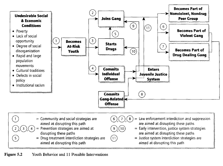
Individual-level logic model. The first type assumes that your case study is about an individual person, with Figure 5.2 depicting the behavioral course of events for a hypothetical youth. The events flow across a series of boxes and arrows reading from left to right in the figure. It suggests that the youth may be at risk for becoming a member of a gang, may eventually join a gang and become involved in gang violence and drugs, and even later may participate in a gang-related criminal offense. Distinctive about this logic model is the series of 11 numbers associated with the various arrows in the figure. Each of the 11 represents an opportunity, through some type of planned intervention (e.g., community or public program), to prevent an individual youth from continu­ing on the course of events. For instance, community development programs (number 1) might bring jobs and better housing to a neighborhood and reduce the youth’s chances of becoming at risk in the first place. How a particular youth might have encountered and dealt with any or all of the 11 possible interventions might be the subject of a case study, with Figure 5.2 helping you to define the relevant data and their analysis.

Firm or organizational-level logic model. A second type of logic model traces events taking place in an individual organization, such as a manufacturing firm. Figure 5.3 shows how changes in a firm (Boxes 5 and 6 in Figure 5.3) are claimed to lead to improved manufacturing (Box 8) and eventually to improved business performance (Boxes 10 and 11). The flow of boxes also reflects a hypothesis—that the initial changes were the result of external bro­kerage and technical assistance services. Given this hypothesis, the logic model therefore also contains rival or competing explanations (Boxes 12 and 13). The data analysis for this case study would then consist of tracing the actual events over time, at a minimum giving close attention to their chrono­logical sequence. The data collection also should have tried to identify ways in which the boxes were actually linked in real life, thereby corroborating the layout of the arrows connecting the boxes.

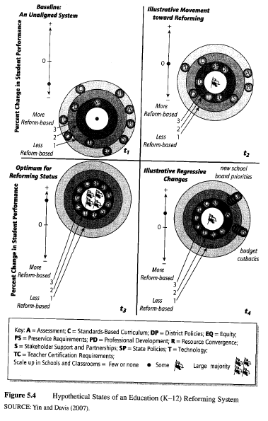
An alternative configuration for an organizational-level logic model. Graphically, nearly all logic models follow a linear sequence (e.g., reading from left to right or from top to bottom). In real life, however, events can be more dynamic, not necessarily progressing linearly. One such set of events might occur in relation to the “reforming” or “transformation” of an organization. For instance, business firms may undergo many significant operational changes, and the business’s mission and culture (and even name) also may change. The sig­nificance of these changes warrants the notion that the entire business has been transformed (see Yin, 2003, chaps. 6 and 10, for a case study of a single firm and then the cross-case analysis of a group of transformed firms). Similarly, schools or school systems can sufficiently alter their way of doing business that “sys­temic reform” is said to be occurring. In fact, major public initiatives deliber­ately aim at improving schools by encouraging the reform of entire school systems (i.e., school districts). However, neither the business transformation nor school reform processes are linear, in at least two ways. First, changes may reverse course and not just progress in one direction. Second, the completed transformation or systemic reform is not necessarily an end point implied by the linear logic model (i.e., the final box in the model); continued transforming and reforming may be ongoing processes even over the long haul.

Figure 5.4 presents an alternatively configured, third type of logic model, reflecting these conditions. This logic model tracks all of the main activities in a school system (the initials are decoded in the key to the figure)—over four periods of time (each time interval might represent a 2- or 3-year period of time). Systemic reform occurs when all of the activities are aligned and work together, and this occurs at t₃ in Figure 5.4. At later stages, however, the reform may regress, represented by t₄, and the logic model does not assume that the vacillations will even end at t₄. As a further feature of the logic model, the entire circle at each stage can be positioned higher or lower, representing the level of student performance—the hypothesis being that systemic reform will be associated with the highest performance. The pennants in the middle of the circle indicate the number of schools or classrooms implementing the desired reform practices, and this number also can vacillate. Finally, the logic model contains a “metric,” whereby the positioning of the activities or the height of the circle can be defined as a result of analyzing actual data.

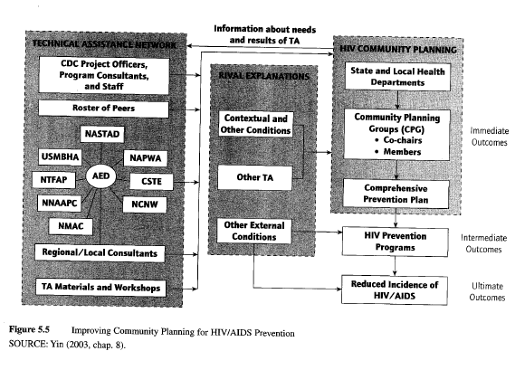
Program-level logic model. Returning to the more conventional linear model, Figure 5.5 contains a fourth and final type of logic model. Here, the model depicts the rationale underlying a major federal program, aimed at reducing the incidence of HIV/AIDS by supporting community planning and prevention initiatives. The program provides funds as well as technical assistance to 65 state and local health departments across the country. The model was used to organize and analyze data from eight case studies, including the collection of data on rival explanations, whose potential role also is shown in the model (see Yin, 2003 chap. 8, for the entire multiple-case study).

Summary. Using logic models represents a fourth technique for analyzing case study data. Four types of logic models, applicable to different units of analysis and situations, have been presented. You should define your logic model prior to collecting data and then “test” the model by seeing how well the data sup­port it (see Yin, 2003, for several examples of case studies using logic models).

5. Cross-Case Synthesis

A fifth technique applies specifically to the analysis of multiple cases (the previous four techniques can be used with either single- or multiple-case stud­ies). The technique is especially relevant if, as advised in Chapter 2, a case study consists of at least two cases (for a synthesis of six cases, see Ericksen & Dyer, 2004). The analysis is likely to be easier and the findings likely to be more robust than having only a single case. BOX 33 presents an excellent example of the important research and research topics that can be addressed by having a “two-case” case study. Again, having more than two cases could strengthen the findings even further.

Cross-case syntheses can be performed whether the individual case studies have previously been conducted as independent research studies (authored by different persons) or as a predesigned part of the same study. In either situa­tion, the technique treats each individual case study as a separate study. In this way, the technique does not differ from other research syntheses—aggregating findings across a series of individual studies (see BOX 34). If there are large numbers of individual case studies available, the synthesis can incorporate quantitative techniques common to other research syntheses (e.g., Cooper & Hedges, 1994) or meta-analyses (e.g., Lipsey, 1992). However, if only a mod­est number of case studies are available, alternative tactics are needed.

One possibility starts with the creation of word tables that display the data from the individual cases according to some uniform framework. Figure 5.6 has an example of such a word table, capturing the findings from 14 case studies of orga­nizational centers, with each center having an organizational partner (COSMOS Corporation, 1998). Of the 14 centers, 7 had received programmatic support and were considered intervention centers; the other 7 were selected as comparison centers. For both types of centers, data were collected about the center’s ability to co-locate (e.g., share facilities) with its partnering organization—this being only one of several outcomes of interest in the original study.

BOX 33

Using a “Two-Case” Case Study to Test a Policy-Oriented Theory

The international marketplace of the 1970s and 1980s was marked by Japan’s promi­nence. Much of its strength was attributable to the role of centralized planning and support by a special governmental ministry—considered by many to be an unfair competitive edge, compared to the policies in other countries. For instance, the United States was considered to have no counterpart support structures. Gregory Hooks’s (1990) excellent case study points to a counterexample frequently ignored by advocates: the role of the U.S. defense department in implementing an industrial planning policy within defense-related industries.

Hooks (1990) provides quantitative data on two cases—the aeronautics industry and the microelectronics industry (the forerunner to the entire computer chip mar­ket and its technologies, such as the personal computer). One industry (aeronautics) has traditionally been known to be dependent upon support from the federal gov­ernment, but the other has not. In both cases, Hooks’s evidence shows how the defense department supported the critical early development of these industries through financial support, the support of R&D, and the creation of an initial cus­tomer base for the industry’s products. The existence of both cases, and not the aero­nautics industry alone, makes the author’s entire argument powerful and persuasive.

BOX 34

Eleven Program Evaluations and a Cross-“Case” Analysis

Dennis Rosenbaum (1986) collected 11 program evaluations as separate chapters in an edited book. The 11 evaluations had been conducted by different investigators, had used a variety of methods, and were not case studies. Each evaluation was about a different community crime prevention intervention, and some presented ample quantitative evidence and employed statistical analyses. The evaluations weie delib­erately selected because nearly all had shown positive results. A cross-case analysis was conducted by the present author (Yin, 1986), treating each evaluation as if it were a separate “case.” The analysis dissected and arrayed the evidence from the 11 evaluations in the form of word tables. Generalizations about successful community crime prevention, independent of any specific intervention, were then derived by using a replication logic, given that all of the evaluations had shown positive results.

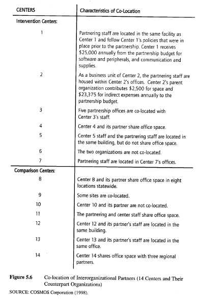
The overall pattern in the word table led to the conclusion that the interven­tion and comparison centers did not differ with regard to this particular out­come. Additional word tables, reflecting other processes and outcomes of interest, were examined in the same way. The analysis of the entire collection of word tables enabled the study to draw cross-case conclusions about the intervention centers and their outcomes.

Complementary word tables can go beyond the single features of a case and array a whole set of features on a case-by-case basis. Now, the analysis can start to probe whether different groups of cases appear to share some similar­ity and deserve to be considered instances of the same “type of general case. Such an observation can further lead to analyzing whether the arrayed case studies reflect subgroups or categories of general cases—raising the possibil­ity of a typology of individual cases that can be highly insightful.

An important caveat in conducting this kind of cross-case synthesis is that the examination of word tables for cross-case patterns will rely strongly on argumentative interpretation, not numeric tallies. Chapter 2 has previously pointed out, however, that this method is directly analogous to cross-experiment interpretations, which also have no numeric properties when only a small number of experiments are available for synthesis. A challenge you must be prepared to meet as a case study investigator is therefore to know how to develop strong, plausible, and fair arguments that are supported by the data.

Source: Yin K Robert (2008), Case Study Research Designs and Methods, SAGE Publications, Inc; 4th edition.