Problem 7.1: Chi-Square and Phi (or Cramer’s V) with SPSS

The statistics discussed in this first problem are designed to analyze two nominal or dichotomous variables. Remember, nominal variables are variables that have distinct unordered levels or categories; each subject is in only one level (you can only be male or female). Chi-square (x2) or phi/Cramer’s V are good choices for statistics when analyzing two nominal variables. They are less appropriate if either variable has three or more ordered levels because these statistics do not take into account the order and thus sacrifice statistical power if used with ordinal or scale variables.

Chi-square requires a relatively large sample size and/or a relatively even split of the subjects among the levels because the expected counts in 80% of the cells should be greater than five. Fisher’s exact test should be reported instead of chi-square for small samples if each of the two variables being related has only two levels (2 x 2 cross-tabulation). Chi-square and the Fisher’s exact test provide similar information about relationships among variables; however, they only tell us whether the relationship is statistically significant (i.e., not likely to be due to chance). They do not tell the effect size (i.e., the strength of the relationship). Another way to interpret chi­square is as a test of whether there are differences between the groups formed from one variable (gender in this problem) on the incidence or counts of each category of the other variable (see Table 6.1).

Phi and Cramer’s V provide a test of statistical significance and also provide information about the strength of the association between two categorical variables. They can be used as measures of the effect size. If one has a 2 x 2 cross-tabulation, phi is the appropriate statistic. For larger cross-tabs, Cramer’s V is used. If one variable has only two categories but the other has more than two categories, then Cramer’s V is equal to phi. The numbers in the cross-tabs description refer to the number of levels in each of the variables. Thus, for gender and religion in the HSB data set, the cross-tab would be 2 x 3 because gender has two levels and religion has three levels.

For phi and Cramer’s V, the strength of association measures belong to the r family of effect sizes and are similar to the correlations you will compute in the next chapter (see Table 6.5). Like correlation, a strong phi or Cramer’s V could be close to 1.00 or -1.00, whereas one close to zero would indicate no relationship. A problem with phi and Cramer’s V is that, under some conditions, the maximum possible value of these statistics is considerably less than 1.00. This makes them hard to interpret.

Assumptions and Conditions for the Use of Chi-square, Phi, Cramer’s V, and Odds Ratios

• The data for the variables must be independent. Each subject is assessed only once.
• Data are treated as nominal, even if ordered.
• For chi-square, if the expected frequencies are less than 5, the test of significance is too liberal. At least 80% of the expected frequencies should be 5 or larger. All should be at least 5 if you have a 2 x 2 chi-square; if they are not, use Fisher’s exact test.
• Odds ratios and risk ratios are problematic to interpret when the probability of an event is near zero (i.e., < .1) or near 1.
  • Do males and females differ on whether they have high or low math grades? If so, how strong is the relationship between gender and high/low math grades?

Let’s see if males and females differ in terms of their math grades. Remember, both the gender and math grades variables are dichotomous; they each have two values.

• Click on Analyze  → Descriptive Statistics → Crosstabs… 
• Move math grades to the Rows box using the arrow key and put gender in the Columns (Where to move these variables is a decision for the researcher. When one of the variables has more levels, it can make interpretation easier if this variable is in the Row(s) box.)

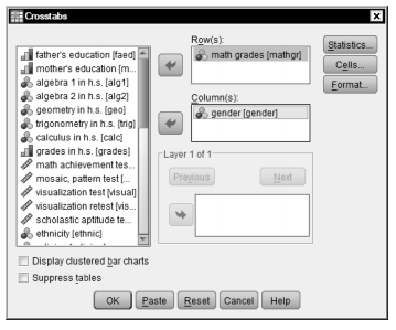
Fig. 7.1. Crosstabs 

• Next, click on Statistics in Fig. 7.1.
• Check Chi-square and Phi and Cramer’s V. The window should look like Figure 7.2.

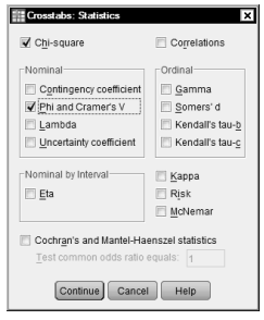
Fig.7.2.Crosstabs statistics.

• Click on Continue.
• Once you return to the Crosstabs menu (Fig. 7.1), click on Cells.
• Now, ensure that Observed is checked; also in Fig. 7.3, check Expected under Counts, and Column under Percentages. It helps the interpretation if the total of the percentages of students for each level of the presumed independent variable (gender, in this case) adds up to 100%. Because gender is the column variable, we checked Column.

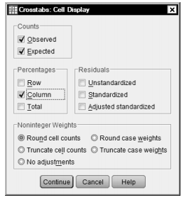
Fig.7.3.Crosstabs: Cell display.

• • Click on Continue, then on OK. Compare your output to Output 7.1.

Output 7.1: Crosstabs With Chi-Square and Phi

CROSSTABS

/TABLES=mathgr BY gender

/FORMAT= AVALUE TABLES

/STATISTICS=CHISQ PHI

/CELLS= COUNT EXPECTED COLUMN

/COUNT ROUND CELL .

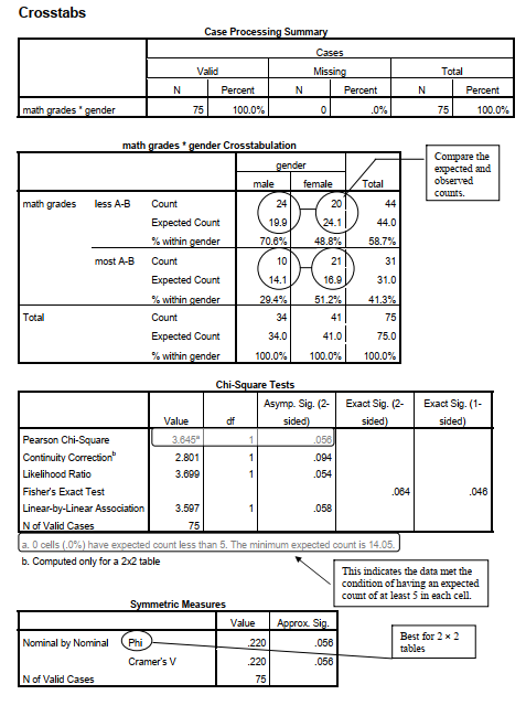
Interpretation of Output 7.1

The case processing summary table indicates that there are no participants with missing data. The Crosstabulation table includes the Counts and Expected Counts, and each cell also has a % within gender. For example, there are 24 males who had low math grades (less than A – B); this is 71% of the 34 male students. On the other hand, 20 of 41 females had low math grades; that is only 49% of the females. It looks like a higher percentage of males had low math grades. The Chi­Square Tests tables tell us whether we can be confident that this apparent difference is not due to chance.

Note, in the Cross-tabulation table, that the Expected Count of the number of male students who had low math grades is 19.9 and the observed or actual Count is 24. Thus, there are 4.1 fewer males who had low math grades than would be expected by chance, given the Totals shown in the table. There are also the same discrepancies between observed and expected counts in the other three cells of the table. A question answered by the chi-square test is whether these discrepancies between observed and expected counts are bigger than one might expect by chance.

The Chi-Square Tests table is used to determine if there is a statistically significant relationship between two dichotomous or nominal variables. It tells you whether the relationship is statistically significant but does not indicate the strength of the relationship, like phi or a correlation does. In Output 7.1, we use the Pearson Chi-Square or (for small samples) the Fisher’s Exact Test to interpret the results of the test. The two-sided (tailed) chi-square test is not statistically significant (p = .056), which indicates that we cannot be certain that males and females are different on whether they have low math grades. Note that in this case the Fisher’s Exact Test leads to different interpretations depending on whether one uses the one-sided column (p = .046, statistically significant) or the two-sided column (p = .064, not significant). You would only use the one-sided column if you had predicted before the study that females would have higher math grades; i.e., your alternative hypothesis was directional. Also note that footnote b states that no cells have expected counts less than 5. That is good because otherwise a condition for using chi-square would be violated. (If so, we could then use the Fisher exact test.) A good guideline is that no more than 20% of the cells should have expected frequencies less than 5. For chi-square with 1 df (i.e., a 2 x 2 cross-tabulation as in this case), none of the cells should have expected frequencies less than 5. Some statisticians say none less than 10.

The Symmetric Measures table provides measures of the strength of the relationships or effect size. If the association between variables is weak, the Value of the statistic will be relatively close to zero. If the relationship or effect size is large, the value should be +/- .50 or more. However, remember that the maximum value for phi and Cramer’s V may be less than 1.00, the theoretical maximum for most measures of association. If both variables have two levels (i.e., 2 x 2 cross-tabs), phi is the appropriate statistic. In Output 7.1, phi is .22, and, like the chi-square, it is not statistically significant. Phi, in this case, is a smaller sized effect than is typical in the behavioral sciences (see Table 6.5) according to Cohen (1988).

Example of How to Write About the Results of Problem 7.1

Results

To investigate whether males and females differ on whether they have high or low math grades, a chi-square statistic was conducted. Assumptions were checked and were met. Table 7.1 shows the Pearson chi-square results and indicates that males and females are not significantly different on whether or not they have high math grades (%² = 3.65, df = 1, N = 75, p =.056). Males are not more likely than expected under the null hypothesis to have low or high math grades than are females. Phi, which indicates the strength of the association between the two variables, is .22.

Source: Morgan George A, Leech Nancy L., Gloeckner Gene W., Barrett Karen C.

(2012), IBM SPSS for Introductory Statistics: Use and Interpretation, Routledge; 5th edition; download Datasets and Materials.