Problem 8.2: Hierarchical Logistic Regression with SPSS

We will rerun Problem 8.1, but this time we will enter the background variables gender and parents’ education first and then, on the second step or block, enter mosaic and visualization test.

• If we control for gender and parents’ education, will mosaic and/or visualization test add to the prediction of whether students will take algebra 2?

Now use the same dependent variable and covariates except enter gender and parents’ education in Block 1 and then enter mosaic and visualization test in Block 2. Use these commands:

• Select Analyze → Regression → Binary Logistic…
• Click on Reset.
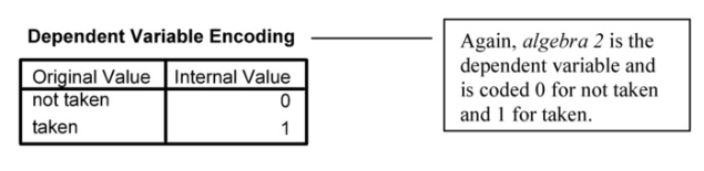
• Move algebra 2 in h.s. into the Dependent: variable box.
• Move gender and parents’ education into the Covariates box (in this problem we actually are treating them as covariates in that we remove variance associated with them first; however, in SPSS all predictors are called Covariates).
• Make sure Enter is the selected Method.
• Click on Next to get Block 2 of 2 (see 8.1 if you need help).
• Move mosaic and visualization test into the Covariates
• Click on Options.
• Check CI for exp(B), and be sure 95 is in the box (which will provide confidence intervals for the odds ratio of each predictor’s contribution to the equation).
• Click on Continue.
• Click on OK. Does your output look like Output 8.2?

Output 8.2: Logistic Regression

LOGISTIC REGRESSION VARIABLES alg2 /METHOD = ENTER gender parEduc

/METHOD = ENTER mosaic visual

/PRINT = CI(95)

/CRITERIA = PIN(.05) POUT(.10) ITERATE(20) CUT(.5) .

Block 0: Beginning Block

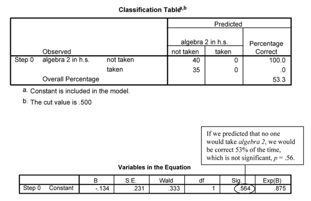
Block 0: Beginning Block

Interpretation of Output 8.2

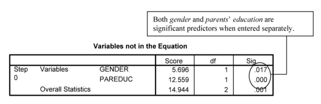
The first four tables are the same as in Output 8.1. In this case, we have an additional step or block (Block 2). Block 1 shows the Omnibus Chi-Square, Model Summary, Classification Table, and Variables in the Equation when gender and parents’ education were entered as covariates. Note that the Omnibus Test is statistically significant (x2 = 16.11, p < .001). With only gender and parents’ education entered, overall we can predict correctly 71% of the cases. Note from the last table in Block 1, that gender is not significant (p = .100) when it and parents’ education are both in the equation.

The log likelihood value (87.53 for Block 1) shows how well the data fit the model. It is similar to the residual sum of squares in multiple regression. The larger the value, the more poorly the model fits.

Block 2: Method=Enter

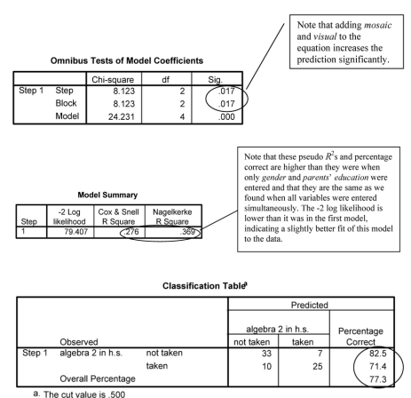
Note that these pseudo /?²s and percentage correct are higher than they were when only gender and parents’ education were entered and that they are the same as we found when all variables were entered simultaneously. The -2 log likelihood is lower than it was in the first model, indicating a slightly better fit of this model to the data.

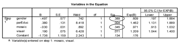
Note that neither gender nor mosaic is significant when all of these variables are entered together.

Source: Leech Nancy L. (2014), IBM SPSS for Intermediate Statistics, Routledge; 5th edition;

download Datasets and Materials.