Problem 10.1: Repeated-Measures ANOVA with SPSS

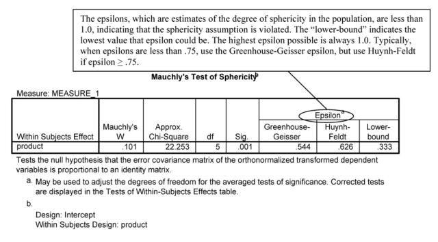
The GLM repeated-measures procedure provides a variety of analysis of variance procedures to use when the same measurement is made several times on each subject or the same measurement is made on several related subjects. The single­factor repeated-measures ANOVA, which we will use for Problem 10.1, is appropriate when you have one independent variable with two or more levels that represent the occasions on which repeated measures were made, the family member who was responding to the questions, or other similar categories involving non-independent assessments of the same outcome variable. If there are only two levels of the independent variable, the sphericity assumption is not a problem because there is only one pair of levels. If between-subjects factors are specified, they divide the sample into groups. There are no between-subjects (also called between-groups) factors in this problem. Finally, you can use a multivariate or univariate approach to testing repeated-measures effects.

• Are there differences among the average ratings for the four products?

Let’s test whether there are differences among the average ratings of the four products. We are assuming the product ratings are scale/normal data. Follow these commands:

• Analyze → General Linear Model → Repeated Measures (see 10.3).
• Delete the factor 1 from the Within-Subject Factor Name box and replace it with the name product, our name for the repeated-measures independent variable that SPSS will generate from the four products.
• Type 4 in the Number of Levels box since there are four products established in the data file.
• Click on Add so the screen looks like 10.3, then click on Define to get Fig. 10.4.

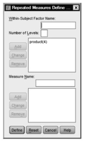
Fig.10.3.Repeated measures GLM define factor(s).

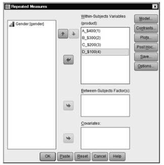
Fig.10.4.GLM repeated measures.

• Now move A_$400, B_$300, C_$200, D_$100 over to the Within-Subjects Variables
• Click on Contrasts. Be sure Polynomial is in the parenthesis after product (see 10.5). SPSS does not provide post hoc tests for the within- subjects (repeated-measures) effects, so we will use contrasts. If the products are ordered, let’s say, by price, we can use the polynomial contrasts that are interpreted below. If we wanted to use a different type of contrast, we could change the type by clicking on the arrow under Change Contrast.
• Click on Continue to get 10.4 again.

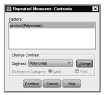
Fig 10.5. Repeated measures: Contrasts.

• Click on Options to get 10.6.
• Click on Descriptive statistics, Estimates of effect size, and Observed power.

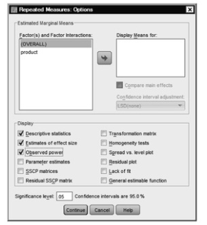
Fig 10.6. Repeated measures: Options.

• Click on Continue, then on OK.

Compare your syntax and output with Output 10.1.

Output 10.1: Repeated-Measures ANOVA Using the General Linear

Model Program

GLM A_$400 B_$300 C_$200 D_$100

/WSFACTOR=Product D Polynomial

/METHOD=SSTYPE(3)

/PRINT=DESCRIPTIVE ETASQ OPOWER

/CRITERIA=ALPHA(.05)

/WSDESIGN=product.

General Linear Model

Interpretation of Output 10.1

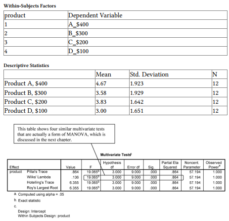
The first table identifies the four levels of the within-subjects, repeated- measures independent variable, product. The second table gives the M and SD for each product on the 1-7 rating, which is the dependent variable.

The third table presents four similar Multivariate Tests of the within- subjects effect (i.e., whether the four products are all rated equally). Wilks’ lambda is a commonly used multivariate test. Notice that in this case, the Fs, df, and significance are the same for each of the multivariate tests: F(3, 9) = 19.07, p < .001. The significant F means that there is a difference somewhere in how the products are rated. The multivariate tests can be used even if sphericity is violated. However, if epsilons are high, indicating that one is close to achieving sphericity, these multivariate tests may be less powerful in the next table (less likely to indicate statistical significance) than the corrected univariate repeated-measures ANOVA shown below. Also note that the observed power is extremely high (1.0); thus it would be possible to have a statistically significant result with a small effect size, which might not be practically meaningful. However, partial eta is very large (7.864 = .93) so this is not an issue.

Source: Leech Nancy L. (2014), IBM SPSS for Intermediate Statistics, Routledge; 5th edition;

download Datasets and Materials.