Application 1: Testing the Factorial Validity of a Theoretical Construct (First-Order CFA Model) with AMO

1. Key Concepts

• Hypothesized models conceptualized within a matrix format
• Error/uniqueness parameters
• Congeneric measures
• Working with model-refining tools in Amos Graphics
• Specification of data in Amos Graphics
• Calculation of estimates in Amos Graphics
• Selection of textual versus graphical output in Amos Graphics
• Evaluation of parameter estimates
• Evaluation of model as a whole
• model-fitting process
• issue of statistical significance in SEM
• estimation process
• goodness-of-fit statistics
• separate computation of standardized RMR
• Issue of model misspecification
• Use and interpretation of modification indices
• Use and interpretation of standardized residuals
• Calculation of standardized root mean square residual
• Post hoc analyses: Justification versus no justification

Our first application examines a first-order CFA model designed to test the multidimensionality of a theoretical construct. Specifically, this application tests the hypothesis that self-concept (SC), for early adolescents (Grade 7), is a multidimensional construct composed of four factors—general SC (GSC), academic SC (ASC), English SC (ESC), and mathematics SC (MSC). The theoretical underpinning of this hypothesis derives from the hierarch­ical model of SC proposed by Shavelson, Hubner, and Stanton (1976). The example is taken from a study by Byrne and Worth Gavin (1996) in which four hypotheses related to the Shavelson et al. model were tested for three groups of children—preadolescents (Grade 3), early adolescents (Grade 7), and late adolescents (Grade 11). Only tests bearing on the multidimen­sional structure of SC, as they relate to grade 7 children, are of interest in the present chapter. This study followed from earlier work in which the same 4-factor structure of SC was tested for adolescents (see Byrne & Shavelson, 1986), and was part of a larger study that focused on the structure of social SC (Byrne & Shavelson, 1996). For a more extensive dis­cussion of the substantive issues and the related findings, readers should refer to the original Byrne and Worth Gavin (1996) article.

2. The Hypothesized Model

At issue in this first application is the plausibility of a multidimensional SC structure for early adolescents. Although numerous studies have sup­ported the multidimensionality of the construct for Grade 7 children, others have counter argued that SC is less differentiated for children in their pre- and early adolescent years (e.g., Harter, 1990). Thus, the argument could be made for a 2-factor structure comprising only GSC and ASC. Still others postulate that SC is a unidimensional structure so that all facets of SC are embodied within a single SC construct (GSC). (For a review of the literature related to these issues, see Byrne, 1996.) The task presented to us here, then, is to test the original hypothesis that SC is a 4-factor structure comprising a general domain (GSC), an academic domain (ASC), and two subject-specific domains (ESC; MSC), against two alternative hypotheses: (a) that SC is a 2-factor structure comprising GSC and ASC, and (b) that SC is a 1-factor structure in which there is no distinction between general and academic SCs.

We turn now to an examination and testing of each of these three hypotheses.

Hypothesis 1: Self-concept is a 4-Factor Structure

The model to be tested in Hypothesis 1 postulates a priori that SC is a 4-factor structure composed of general SC (GSC), academic SC (ASC), English SC (ESC), and math SC (MSC); it is presented schematically in Figure 3.1.

Prior to any discussion of how we might go about testing this model, let’s take a few minutes first to dissect the model and list its component parts as follows:

• There are four SC factors, as indicated by the four ellipses labeled GSC, ASC, ESC, and MSC.
• These four factors are intercorrelated, as indicated by the two-headed arrows.
• There are 16 observed variables, as indicated by the 16 rectangles (SDQ2N01-SDQ2N43); they represent item-pairs from the General, Academic, Verbal, and Math SC subscales of the Self Description Questionnaire II (Marsh, 1992a).

• The observed variables load on the factors in the following pat­tern: SDQ2N01-SDQ2N37) load on Factor 1; SDQ2N04-SDQ2N40 load on Factor 2; SDQ2N10-SDQ2N46 load on Factor 3; and SDQ2N07-SDQ2N42 load on Factor 4.
• Each observed variable loads on one and only one factor.
• Errors of measurement associated with each observed variable (err01-err43) are uncorrelated.

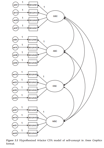
Summarizing these observations, we can now present a more formal description of our hypothesized model. As such, we state that the CFA model presented in Figure 3.1 hypothesizes a priori that

• SC responses can be explained by four factors: GSC, ASC, ESC, and MSC.
• Each item-pair measure has a nonzero loading on the SC factor that it was designed to measure (termed a “target loading”), and a zero-loading on all other factors (termed “nontarget loadings”).
• The four SC factors, consistent with the theory, are correlated.
• Error/uniquenesses¹ associated with each measure are uncorrelated.

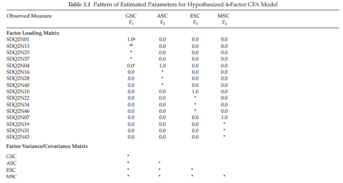
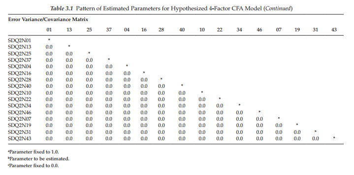
Another way of conceptualizing the hypothesized model in Figure 3.1 is within a matrix framework as presented in Table 3.1. Thinking about the model components in this format can be very help­ful because it is consistent with the manner in which the results from SEM analyses are commonly reported in program output files. Although Amos, as well as other Windows-based programs, also provides users with a graphical output, the labeled information is typically limited to the estimated values and their standard errors. The tabular represen­tation of our model in Table 3.1 shows the pattern of parameters to be estimated within the framework of three matrices: the factor loading matrix, the factor variance/covariance matrix, and the error variance/ covariance matrix. For purposes of model identification and latent vari­able scaling (see Chapter 2), you will note that the first of each con­generic² set of SC measures in the factor loading matrix is set to 1.0; all other parameters are freely estimated (as represented by an asterisk [*]). Likewise, as indicated by the asterisks appearing in the variance/ covariance matrix, all parameters are to be freely estimated. Finally, in the error/uniqueness matrix, only the error variances are estimated; all error covariances are presumed to be zero.

3. Modeling with Amos Graphics

Provided with these two perspectives of the hypothesized model, let’s now move on to the actual testing of the model. We’ll begin by examining the route to model specification, data specification, and the calculation of parameter estimates within the framework of Amos Graphics.

Model Specification

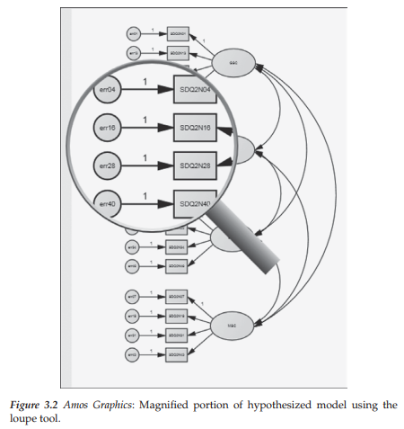
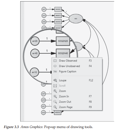
The beauty of working with the Amos Graphics interface is that all we need to do is to provide the program with a hypothesized model; in the present case, we use the one portrayed in Figure 3.1. Given that I demonstrated most of the commonly-used drawing tools, and their application, in Chapter 2, there is no need for me to walk you through the construction of this model here. Likewise, construction of hypoth­esized models presented throughout the remainder of the book will not be detailed. Nonetheless, I take the opportunity, wherever possible, to illustrate a few of the other drawing tools or features of Amos Graphics not specifically demonstrated earlier. Accordingly, in the last two edi­tions of this book, I noted two tools that, in combination, I had found to be invaluable in working on various parts of a model; these were the Magnification ]§] and the Scroll H tools. To use this approach in modify­ing graphics in a model, you first click on the Magnification icon, with each click enlarging the model slightly more than as shown in the pre­vious view. Once you have achieved sufficient magnification, you then click on the Scroll icon to move around the entire diagram. Clicking on the Reduction tool SI would then return the diagram to the normal view. You can also zoom in on specific objects of a diagram by simply using the mouse wheel. Furthermore, the mouse wheel can also be used to adjust the magnification of the Loupe tool Although the Scroll tool enables you to move the entire path diagram around, you can also use the scrollbars that appear when the diagram extends beyond the Amos Graphics window. An example of magnification using the Loupe tool is presented in Figure 3.2. Finally, it is worth noting that when either the Scroll, Magnification, or Loupe tools are activated, a right-click of the mouse will provide a pop-up menu of different diagram features you may wish to access (see Figure 3.3).

Data Specification

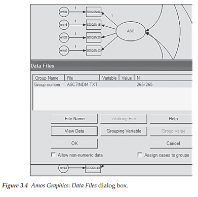
Now that we have provided Amos with the model to be analyzed, our next job is to tell the program where to find the data. All data to be used in applications throughout this book have been placed in an Amos folder called “Data Files.” To activate this folder, we can either click on the Data File icon g§], or pull down the File menu and select “Data Files.” Either choice will trigger the Data Files dialog box displayed in Figure 3.4; it is shown here as it pops up in the forefront of your workspace.

In reviewing the upper section of this dialog box, you will see that the program has identified the Group Name as “Group number 1”; this labeling is default in the analysis of single sample data. The data file to be used for the current analysis is labeled “ASC7INDM.TXT,” and the sam­ple size is 265; the 265/265 indicates that, of a total sample size of 265, 265 cases have been selected for inclusion in the analysis. In the lower half of the dialog box, you will note a View Data button that allows you to peruse the data in spreadsheet form should you wish to do so. Once you have selected the data file that will serve as the working file upon which your hypothesized model is based, you simply click the OK button.

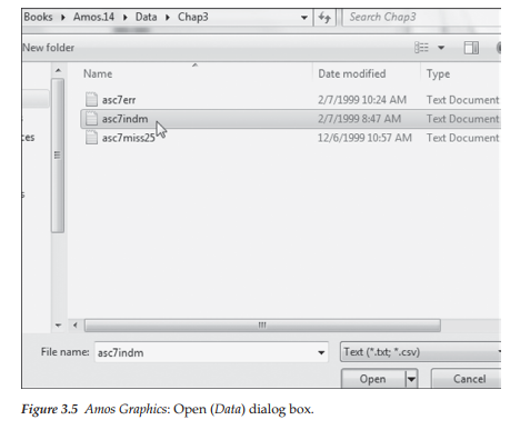
In the example shown here, the selected data file was already visible in the Data Files dialog box. However, suppose that you needed to select this file from a list of several available data sets. To do so, you would click on the File Name button in the Data Files dialog box (see Figure 3.4). This action would then trigger the Open dialog box shown in Figure 3.5. Here, you select a data file and then click on the Open button. Once you have opened a file, it becomes the working file and its filename will then appear in the Data Files dialog box, as illustrated in Figure 3.4.

It is important that I point out some of the requirements of the Amos program in the use of external data sets. If your data files are in ASCII format, you may need to restructure them before you are able to conduct any analyses using Amos. Consistent with SPSS and many other Windows applications, Amos requires that data be structured in tab-delimited (as well as comma- or semicolon-delimited) text format. Thus, whereas the semicolon (rather than the comma) delimiter is used in many European and Asian countries, this is not a problem as Amos can detect which version of the program is running (e.g., French version) and then auto­matically defines a compatible delimiter. In addition, all data must res­ide in an external file. The data used in this chapter are in the form of a tab-delimited (.dat) text file. However, Amos supports several common database formats, including SPSS *.sav and Excel *.xl; I use all three text formatted data sets in this book.

Calculation of Estimates

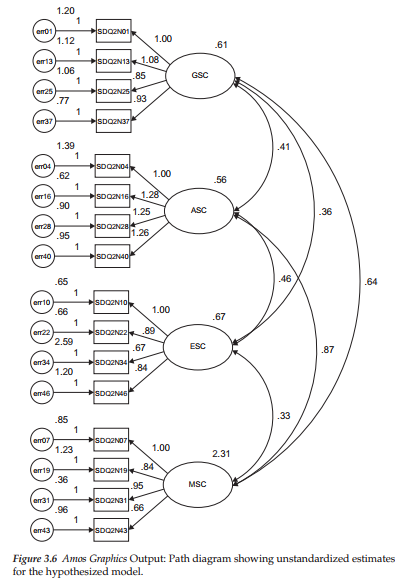
Now that we have specified both the model to be analyzed and the data file upon which the analyses are to be based, all that is left for us to do is to execute the job; we do so by clicking on the Calculate Estimates icon H|. (Alternatively, we could select “Calculate Estimates” from the Analyze drop-down menu.) Once the analyses have been completed, Amos Graphics allows you to review the results from two different perspectives—graphical and textual. In the graphical output, all estimates are presented in the path diagram. These results are obtained by clicking on the View Output Path Diagram icon 0 found at the top of the middle section of the Amos main screen. Results related to the testing of our hypothesized model are pre­sented in Figure 3.6, with the inserted values representing the nonstand- ardized estimates. To copy the graphical output to another file, such as a Word document, either click on the Duplication icon or pull down the Edit menu and select “Copy (to Clipboard).” You can then paste the out­put into the document.

Likewise, you have two methods of viewing the textual output—either by clicking on the Text Output icon m, or by selecting “Text Output” from the View drop-down menu. However, in either case, as soon as the analyses are completed, a red tab representing the Amos output file will appear on the bottom status bar of your computer screen. Let’s turn now to the out­put resulting from our test of the hypothesized model.

Amos Text Output: Hypothesized 4-Factor Model

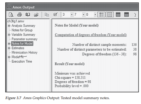
Textual output pertinent to a particular model is presented very neatly in the form of summaries related to specific sections of the output file. This tree-like arrangement enables the user to select out sections of the output that are of particular interest. Figure 3.7 presents a view of this tree-like formation of summaries, with summary information related to the hypothesized 4-factor model open. To facilitate the presentation and discussion of results in this chapter, the material is divided into three pri­mary sections: (a) Model Summary, (b) Model Variables and Parameters, and (c) Model Evaluation.

Model Summary

This very important summary provides you with a quick overview of the model, including the information needed in determining its identification status. Here we see that there are 136 distinct sample moments or, in other words, elements in the sample covariance matrix (i.e., number of pieces of information provided by the data), and 38 parameters to be estimated, leaving 98 degrees of freedom based on an overidentified model, and a chi-square value of 158.511 with probability level equal to .000.

Recall that the only data with which we have to work in SEM are the observed variables, which in the present case number 16. Based on the formula, p(p + 1)/2 (see Chapter 2), the sample covariance matrix for these data should yield 136 (16[17]/2) sample moments, which indeed, it does. A more specific breakdown of the estimated parameters is presented in the Model Variables and Parameters section discussed next. Likewise, an elaboration of the ML (maximum likelihood) chi-square statistic, together with substantially more information related to model fit, is presented and discussed in the Model Evaluation section.

Model Variables and Parameters

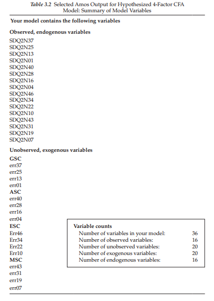
The initial information provided for the Amos text output file can be invalu­able in helping you resolve any difficulties with the specification of a model. The first set of important information is contained in the output file labeled Variable Summary. As shown in Table 3.2, here you will find all the vari­ables in the model (observed and latent), accompanied by their categoriza­tion as either observed or unobserved, and as endogenous or exogenous. Consistent with the model diagram in Figure 3.1, all the observed variables (i.e., the input data) operate as dependent (i.e., endogenous) variables in the model; all factors and error terms are unobserved, and operate as independ­ent (i.e., exogenous) variables in the model. This information is followed by a summary of the total number of variables in the model, as well as the number in each of the four categories, shown in the boxed area in Table 3.2.

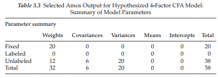
The next section of the output file, listed as Parameter Summary, focuses on a summary of the parameters in the model and is presented in Table 3.3. Moving from left to right by column, we see that there are 32 regression weights, 20 of which are fixed and 12 of which are estimated; the 20 fixed regression weights include the first of each set of 4 factor loadings and the 16 error terms. There are 6 covariances and 20 variances, all of which are estimated. In total, there are 58 parameters, 38 of which are to be esti­mated. Provided with this summary, it is now easy for you to determine the appropriate number of degrees of freedom and, ultimately, whether or not the model is identified. Although, of course this information is pro­vided by the program as noted in Figure 3.7, it is always good (and fun?) to see if your calculations are consistent with those of the program.

Model Evaluation

Of primary interest in structural equation modeling is the extent to which a hypothesized model “fits” or, in other words, adequately describes the sample data. Given findings of an inadequate goodness-of-fit, the next logical step is to detect the source of misfit in the model. Ideally, evaluation of model fit should derive from a variety of perspectives and be based on several criteria that assess model fit from a diversity of perspectives. In particular, these evaluation criteria focus on the adequacy of (a) the par­ameter estimates, and (b) the model as a whole.

Parameter Estimates

In reviewing the model parameter estimates, three criteria are of inter­est: (a) the feasibility of the parameter estimates, (b) the appropriateness of the standard errors, and (c) the statistical significance of the parameter estimates. We turn now to a brief explanation of each.

Feasibility of parameter estimates. The initial step in assessing the fit of individual parameters in a model is to determine the viability of their esti­mated values. In particular, parameter estimates should exhibit the correct sign and size, and be consistent with the underlying theory. Any estimates falling outside the admissible range signal a clear indication that either the model is wrong or the input matrix lacks sufficient information. Examples of parameters exhibiting unreasonable estimates are correlations >1.00, negative variances, and covariance or correlation matrices that are not positive definite.

Appropriateness of standard errors. Standard errors reflect the precision with which a parameter has been estimated, with small values suggesting accurate estimation. Thus, another indicator of poor model fit is the pres­ence of standard errors that are excessively large or small. For example, if a standard error approaches zero, the test statistic for its related param­eter cannot be defined (Bentler, 2005). Likewise, standard errors that are extremely large indicate parameters that cannot be determined (Joreskog & Sorbom, 1993).³ Because standard errors are influenced by the units of measurement in observed and/or latent variables, as well as the magni­tude of the parameter estimate itself, no definitive criterion of “small” and “large” has been established (see Joreskog & Sorbom, 1989).

Statistical significance of parameter estimates. The test statistic as reported in the Amos output is the critical ratio (C.R.), which represents the par­ameter estimate divided by its standard error; as such, it operates as a z-statistic in testing that the estimate is statistically different from zero. Based on a probability level of .05, then, the test statistic needs to be >±1.96 before the hypothesis (that the estimate equals 0.0) can be rejected. Nonsignificant parameters, with the exception of error variances, can be considered unimportant to the model; in the interest of scientific parsi­mony, albeit given an adequate sample size, they should be deleted from the model. On the other hand, it is important to note that nonsignifi­cant parameters can be indicative of a sample size that is too small (K.G. Joreskog, personal communication, January, 1997).

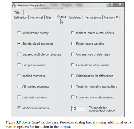
Before we review this section of the Amos output, it is important to alert you that, by default, the program does not automatically include either the standardized parameter estimates or the modification indices (MIs; indicators of misfitting parameters in the model). This requested information must be conveyed to the program prior to proceeding with the calculation of the estimates. Because these additionally esti­mated values can be critically important in determining the adequacy of tested models, I requested this information prior to running the ana­lyses under review here. To request this additional output information, you first either click on the Analysis Properties icon IHD, or select Analysis Properties from the View drop-down menu. Immediately upon clicking on Analysis Properties, you will be presented with the dialog box shown in Figure 3.8 in which the boxes associated with “Standardized estimates” and “Modification indices” have already been checked. Note, also, that I have entered the numeral 10 in the box representing the “Threshold for modification indices,” which I will explain later in my discussion of modification indices.

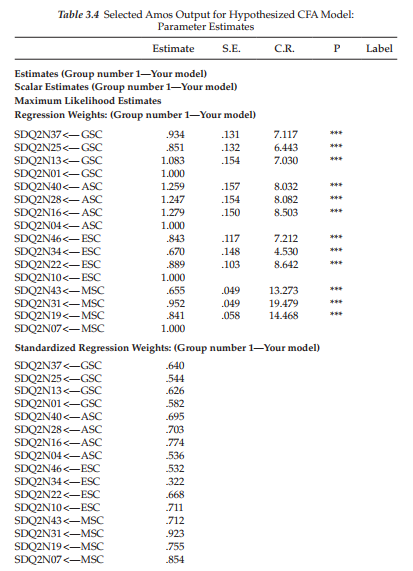
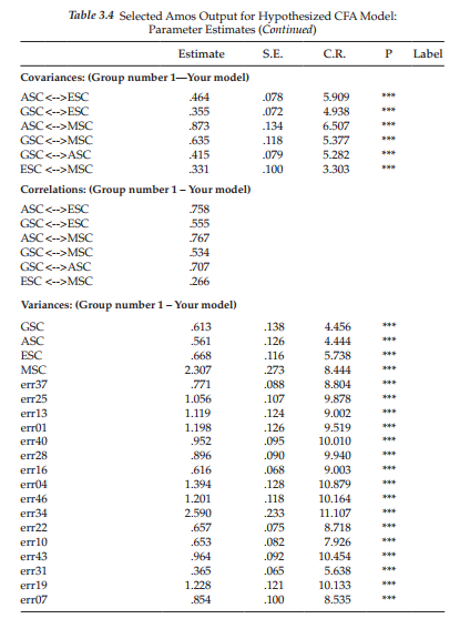
Let’s turn now to this section of the Amos output file. After selecting Estimates from the list of output sections (see Figure 3.7), you will be pre­sented with the information shown in Table 3.4. As you can readily see, results are presented separately for the Factor Loadings (listed as Regression weights), the Covariances (in this case, for factors only), and the Variances (for both factors and measurement errors), with both the unstandardized and standardized estimates being reported. Parameter estimation infor­mation is presented very clearly and succinctly in the Amos text output file. Listed to the right of each parameter is its estimated value (Column 1), standard error (Column 2), critical ratio (Column 3), and probability value (Column 4). An examination of the unstandardized solution reveals all estimates to be reasonable, their standard errors to be low, and their crit­ical ratios to be real, strong evidence of their strong statistical significance.

Model as a Whole

In the Model Summary presented in Figure 3.7, we observed that Amos provided the overall x² value, together with its degrees of freedom and probability value. However, this information is intended only as a quick overview of model fit. Indeed, the program, by default, provides many other fit statistics in its output file. Before turning to this section of the Amos output, however, it is essential that I first review four important aspects of fitting hypothesized models; these are (a) the model-fitting pro­cess, (b) the issue of statistical significance, (c) the estimation process, and (d) the goodness-of-fit statistics.

The model-fitting process. In Chapter 1, I presented a general descrip­tion of this process and noted that the primary task is to determine goodness-of-fit between the hypothesized model and the sample data. In other words, the researcher specifies a model and then uses the sample data to test the model.

With a view to helping you gain a better understanding of the goodness-of-fit statistics presented in the Amos Output file, let’s take a few moments to recast this model-fitting process within a more formal­ized framework. For this, let S represent the sample covariance matrix (of observed variable scores), Z (sigma) represent the population covari­ance matrix, and 9 (theta) represent a vector that comprises the model parameters. Thus, Z(9) represents the restricted covariance matrix implied by the model (i.e., the specified structure of the hypothesized model). In SEM, the null hypothesis (H₀) being tested is that the postulated model holds in the population [i.e., Z = Z(9)]. In contrast to traditional statis­tical procedures, however, the researcher hopes not to reject H₀ (but see MacCallum, Browne, & Sugawara [1996] for proposed changes to this hypothesis-testing strategy).

The issue of statistical significance. The rationale underlying the prac­tice of statistical significance testing has generated a plethora of criti­cism over, at least, the past four decades. Indeed, Cohen (1994) has noted that, despite Rozeboom’s (1960) admonition more than 55 years ago that “the statistical folkways of a more primitive past continue to dominate the local scene” (p. 417), this dubious practice still persists. (For an array of supportive, as well as opposing views with respect to this article, see the American Psychologist [1995], 50, 1098-1103.) In light of this historical bank of criticism, together with the current pressure by methodologists to cease this traditional ritual (see, e.g., Cohen, 1994; Kirk, 1996; Schmidt, 1996; Thompson, 1996), the Board of Scientific Affairs for the American Psychological Association recently appointed a task force to study the feasibility of phasing out the use of null hypothesis testing procedures, as described in course texts and reported in journal articles. Consequently, the end of statistical significance testing relative to traditional statistical methods may soon be a reality. (For a compendium of articles addressing this issue, see Harlow, Mulaik, & Steiger, 1997.)

Statistical significance testing with respect to the analysis of covariance structures, however, is somewhat different in that it is driven by degrees of freedom involving the number of elements in the sample covariance matrix and the number of parameters to be estimated. Nonetheless, it is interesting to note that many of the issues raised with respect to the trad­itional statistical methods (e.g., practical significance, importance of con­fidence intervals, importance of replication) have long been addressed in SEM applications. Indeed, it was this very issue of practical “nonsig­nificance” in model testing that led Bentler and Bonett (1980) to develop one of the first subjective indices of fit (the NFI); their work subsequently spawned the development of numerous additional practical indices of fit, many of which are included in the Amos output. Likewise, the early work of Steiger (1990; Steiger & Lind, 1980) precipitated the call for use of con­fidence intervals in the reporting of SEM findings (see, e.g., MacCallum et al., 1996). Finally, the classic paper by Cliff (1983) denouncing the pro­liferation of post hoc model fitting, and criticizing the apparent lack of concern for the dangers of overfitting models to trivial effects arising from capitalization on chance factors, spirited the development of evaluation indices (Browne & Cudeck, 1989; Cudeck & Browne, 1983), as well as a general call for increased use of cross-validation procedures (see, e.g., MacCallum et al., 1992,1994).

The estimation process. The primary focus of the estimation process in SEM is to yield parameter values such that the discrepancy (i.e., residual) between the sample covariance matrix S and the population covariance matrix implied by the model [Σ(θ)] is minimal. This objective is achieved by minimizing a discrepancy function, F[S, Σ(θ)], such that its minimal value (f_min) reflects the point in the estimation process where the discrepancy between S and Σ(θ) is least [S – Σ(θ) = minimum]. Taken together, then, F_min serves as a measure of the extent to which S differs from Σ(θ).

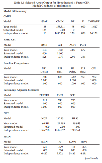
Goodness-of-fit statistics. Let’s now turn to the goodness-of-fit statis­tics that are presented in Table 3.5. This information, as for the param­eter estimates, is taken directly from the Amos output. For each set of fit statistics, you will note three rows. The first row, as indicated, focuses on the Hypothesized model under test (i.e., Your Model), the second on the Saturated model, and the third on the Independence model. Explanation of the latter two models, I believe, is most easily understood within a com­parative framework. As such, think of these three models as representing points on a continuum, with the Independence model at one extreme, the Saturated model at the other extreme, and the Hypothesized model some­where in between. The Independence model is one of complete independ­ence of all variables in the model (i.e., in which all correlations among variables are zero) and is the most restricted. In other words, it is a null model, with nothing going on here as each variable represents a factor. The Saturated model, on the other hand, is one in which the number of estimated parameters equals the number of data points (i.e., variances and covariances of the observed variables, as in the case of the just-identified model), and is the least restricted.

For didactic as well as space reasons, all goodness-of-fit statistics are provided only for the initially hypothesized model in this first application; for all remaining chapters, only those considered to be the most critical in EM analyses will be reported. We turn now to an examination of each cluster, as they relate to the Hypothesized model only. (Formulae related to each fit statistic can be found in Arbuckle, 2012.)

Focusing on the first set of fit statistics, we see the labels NPAR (number of parameters), CMIN (minimum discrepancy), DF (degrees of freedom), P (probability value), and CMIN/DF. The value of 158.511, under CMIN, represents the discrepancy between the unrestricted sam­ple covariance matrix S, and the restricted covariance matrix 1(9) and, in essence, represents the Likelihood Ratio Test statistic, most com­monly expressed as a chi-square (x²) statistic. It is important to note that, for the remainder of the book, I refer to CMIN as x². This statistic is equal to (N – 1)F_min (sample size minus 1, multiplied by the minimum fit function) and, in large samples, is distributed as a central x² with degrees of freedom equal to 1/2(p)(p + 1) – t, where p is the number of observed variables, and t is the number of parameters to be estimated (Bollen, 1989a). In general, H₀: Z = 1(8) is equivalent to the hypothesis that Z – Z(8) = 0; the x² test, then, simultaneously tests the extent to which all residuals in Z – Z(8) are zero (Bollen, 1989a). Framed a little differently, the null hypothesis (H₀) postulates that specification of the factor loadings, factor variances/covariances, and error variances for the model under study are valid; the x² test simultaneously tests the extent to which this specification is true. The probability value associ­ated with x² represents the likelihood of obtaining a x² value that exceeds the x² value when H₀ is true. Thus, the higher the probability associated with x², the closer the fit between the hypothesized model (under H₀) and the perfect fit (Bollen, 1989a).

The test of our H₀, that SC is a 4-factor structure as depicted in Figure 3.1, yielded a x² value of 158.51, with 98 degrees of freedom and a probability of less than .0001 (p < .0001), suggesting that the fit of the data to the hypothesized model is not entirely adequate. Interpreted lit­erally, this test statistic indicates that, given the present data, the hypoth­esis bearing on SC relations, as summarized in the model, represents an unlikely event (occurring less than one time in a thousand under the null hypothesis) and should be rejected.

However, both the sensitivity of the Likelihood Ratio Test to sam­ple size and its basis on the central x² distribution, which assumes that the model fits perfectly in the population (i.e., that H₀ is correct), have led to problems of fit that are now widely known. Because the x² statis­tic equals (N – 1)F_min, this value tends to be substantial when the model does not hold and sample size is large (Joreskog & Sorbom, 1993). Yet, the analysis of covariance structures is grounded in large sample theory. As such, large samples are critical to the obtaining of precise parameter esti­mates, as well as to the tenability of asymptotic distributional approxima­tions (MacCallum et al., 1996). Thus, findings of well-fitting hypothesized models, where the x² value approximates the degrees of freedom, have proven to be unrealistic in most SEM empirical research. More common are findings of a large x² relative to degrees of freedom, thereby indicat­ing a need to modify the model in order to better fit the data (Joreskog & Sorbom, 1993). Thus, results related to the test of our hypothesized model are not unexpected. Indeed, given this problematic aspect of the Likelihood Ratio Test, and the fact that postulated models (no matter how good) can only ever fit real-world data approximately and never exactly, MacCallum et al. (1996) recently proposed changes to the traditional hypothesis-testing approach in covariance structure modeling. (For an extended discussion of these changes, readers are referred to MacCallum et al., 1996.)

Researchers have addressed the x² limitations by developing good- ness-of-fit indices that take a more pragmatic approach to the evaluation process. Indeed, the past three decades have witnessed a plethora of newly developed fit indices, as well as unique approaches to the model­fitting process (for reviews see, e.g., Gerbing & Anderson, 1993; Hu & Bentler, 1995; Marsh, Balla, & McDonald, 1988; Tanaka, 1993). One of the first fit statistics to address this problem was the x²/degrees of free­dom ratio (Wheaton, Muthen, Alwin, & Summers, 1977) which appears as CMIN/DF, and is presented in the first cluster of statistics shown in Table 3.5.⁴ For the most part, the remainder of the Amos output file is devoted to these alternative indices of fit, and, where applicable, to their related confidence intervals. These criteria, commonly referred to as “subjective,” “practical,” or “ad hoc” indices of fit, are typically used as adjuncts to the x² statistic.

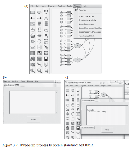
Turning now to the next group of statistics, we see the labels, RMR, GFI, AGFI, and PGFI. The Root Mean Square Residual (RMR) represents the average residual value derived from the fitting of the variance-covariance matrix for the hypothesized model I(9) to the variance-covariance matrix of the sample data (S). However, because these residuals are relative to the sizes of the observed variances and covariances, they are difficult to inter­pret. Thus, they are best interpreted in the metric of the correlation matrix (Hu & Bentler, 1995; Joreskog & Sorbom, 1989). The standardized RMR (SRMR), then, represents the average value across all standardized residu­als, and ranges from zero to 1.00; in a well-fitting model this value will be small, say, .05 or less. The value of .103 shown in Table 3.5 represents the unstandardized residual value. Not shown on the output, however, is the SRMR value. Although this standardized coefficient is typically reported in the output file by other SEM programs, for some reason this is not the case with Amos. Nonetheless, this standardized value can be obtained in a three-step process. First, click on the tab labeled “Plug-ins” located at the top of the Amos Graphics opening page, which will then yield a drop-down menu where you will find “standardized RMR” as the last item listed. Second, click on “standardized RMR,” which then presents you with a blank screen. Finally, with the blank screen open, click on the “Calculate Estimates” icon. Once Amos has calculated this value it will appear in the blank screen. These three steps are shown in Figure 3.9, with the stand­ardized RMR shown to be .0479. It can be interpreted as meaning that the model explains the correlations to within an average error of .048 (see Hu & Bentler, 1995).

The Goodness-of-fit Index (GFI) is a measure of the relative amount of variance and covariance in S that is jointly explained by I. The AGFI differs from the GFI only in the fact that it adjusts for the number of degrees of freedom in the specified model. As such, it also addresses the issue of parsimony by incorporating a penalty for the inclusion of additional parameters. The GFI and AGFI can be classified as absolute indices of fit because they basically compare the hypothesized model with no model at all (see Hu & Bentler, 1995). Although both indices range from zero to 1.00, with values close to 1.00 being indicative of good fit, Joreskog and Sorbom (1993) note that, theoretically, it is possible for them to be negative; Fan, Thompson, and Wang (1999) further caution that GFI and AGFI values can be overly influenced by sample size. This, of course, should not occur as it would reflect the fact that the model fits worse than no model at all.

Based on the GFI and AGFI values reported in Table 3.5 (.933 and .906, respectively) we can once again conclude that our hypothesized model fits the sample data fairly well.

The last index of fit in this group, the Parsimony Goodness-of-fit Index (PGFI), was introduced by James, Mulaik, and Brett (1982) to address the issue of parsimony in SEM. As the first of a series of “parsimony-based indices of fit” (see Williams & Holahan, 1994), the PGFI takes into account the complexity (i.e., number of estimated parameters) of the hypothesized model in the assessment of overall model fit. As such, “two logically interdependent pieces of information,” the goodness-of-fit of the model (as measured by the GFI) and the parsimony of the model, are repre­sented by the single index PGFI, thereby providing a more realistic evalu­ation of the hypothesized model (Mulaik et al., 1989, p. 439). Typically, parsimony-based indices have lower values than the threshold level gen­erally perceived as “acceptable” for other normed indices of fit. Mulaik et al. suggested that nonsignificant x² statistics and goodness-of-fit indices in the .90s, accompanied by parsimonious-fit indices in the 50s, are not unexpected. Thus, our finding of a PGFI value of .672 would seem to be consistent with our previous fit statistics.

We turn now to the next set of goodness-of-fit statistics (Baseline Comparisons), which can be classified as incremental or comparative indi­ces of fit (Hu & Bentler, 1995; Marsh et al., 1988). As with the GFI and AGFI, incremental indices of fit are based on a comparison of the hypothesized model against some standard. However, whereas this standard represents no model at all for the GFI and AGFI, it represents a baseline model (typ­ically the independence or null model noted above for the incremental indices).⁵ We now review these incremental indices.

For the better part of a decade, Bentler and Bonett’s (1980) Normed Fit Index (NFI) has been the practical criterion of choice, as evidenced in large part by the current “classic” status of its original paper (see Bentler, 1992; Bentler & Bonett, 1987). However, addressing evidence that the NFI has shown a tendency to underestimate fit in small samples, Bentler (1990) revised the NFI to take sample size into account and proposed the Comparative Fit Index (CFI; see last column). Values for both the NFI and CFI range from zero to 1.00 and are derived from the compari­son of a hypothesized model with the independence (or null) model, as described earlier. As such, each provides a measure of complete covari­ation in the data, Although a value >.90 was originally considered rep­resentative of a well-fitting model (see Bentler, 1992), a revised cutoff value close to .95 has recently been advised (Hu & Bentler, 1999). Both indices of fit are reported in the Amos output; however, Bentler (1990) has suggested that, of the two, the CFI should be the index of choice. As shown in Table 3.5, the CFI (.962) indicated that the model fitted the data well in the sense that the hypothesized model adequately described the sample data. In somewhat less glowing terms, the NFI value sug­gested that model fit was only marginally adequate (.907). The Relative Fit Index (RFI; Bollen, 1986) represents a derivative of the NFI; as with both the NFI and CFI, the RFI coefficient values range from zero to 1.00, with values close to .95 indicating superior fit (see Hu & Bentler, 1999). The Incremental Index of Fit (IFI) was developed by Bollen (1989b) to address the issues of parsimony and sample size which were known to be associated with the NFI. As such, its computation is basically the same as the NFI, with the exception that degrees of freedom are taken into account. Thus, it is not surprising that our finding of IFI of .962 is consistent with that of the CFI in reflecting a well-fitting model. Finally, the Tucker-Lewis Index (TLI; Tucker & Lewis, 1973), consistent with the other indices noted here, yields values ranging from zero to 1.00, with values close to .95 (for large samples) being indicative of good fit (see Hu & Bentler, 1999).

The next cluster of fit indices all relate to the issue of model parsi­mony. The first fit index (PRATIO) relates to the initial parsimony ratio proposed by James et al. (1982). More appropriately, however, the index has subsequently been tied to other goodness-of-fit indices (see, e.g., the PGFI noted earlier). Here, it is computed relative to the NFI and CFI. In both cases, as was true for PGFI, the complexity of the model is taken into account in the assessment of model fit (see James et al., 1982; Mulaik et al., 1989). Again, a PNFI of .740 and PCFI of .785 (see Table 3.5) fall in the range of expected values.⁶

The next set of fit statistics provides us with the Noncentrality param­eter (NCP) estimate. In our initial discussion of the x² statistic, we focused on the extent to which the model was tenable and could not be rejected. Now, however, let’s look a little more closely at what happens when the hypothesized model is incorrect [i.e., Z * Z(9)]. In this circumstance, the x² statistic has a noncentral x² distribution, with a noncentrality param­eter, A, that is estimated by the noncentrality parameter (Bollen, 1989a; Hu & Bentler, 1995; Satorra & Saris, 1985). The noncentrality parameter is a fixed parameter with associated degrees of freedom, and can be denoted as x²(_df,_A). Essentially, it functions as a measure of the discrepancy between I and 1(0) and, thus, can be regarded as a “population badness-of-fit” (Steiger, 1990). As such, the greater the discrepancy between I and I(0), the larger the A value. (For a presentation of the various types of error associated with discrepancies among matrices, see Browne & Cudeck, 1993; Cudeck & Henly, 1991; MacCallum et al., 1994.) It is now easy to see that the central x² statistic is a special case of the noncentral x² distribution when A = 0.0. (For an excellent discussion and graphic portrayal of dif­ferences between the central and noncentral x² statistics, see MacCallum et al., 1996.) As a means to establishing the precision of the noncentrality parameter estimate, Steiger (1990) has suggested that it be framed within the bounds of confidence intervals. Turning to Table 3.5, we find that our hypothesized model yielded a noncentrality parameter of 60.511. This value represents the x² value minus its degrees of freedom (158.51 – 98). The confidence interval indicates that we can be 90% confident that the population value of the noncentrality parameter (A) lies between 29.983 and 98.953.

For those who may wish to use this information, values related to the minimum discrepancy function (FMIN) and the population discrep­ancy (FO) are presented next. The columns labeled LO90 and HI90 con­tain the lower and upper limits, respectively, of a 90% confidence interval around FO.

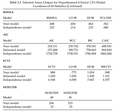
The next set of fit statistics focus on the Root Mean Square Error of Approximation (RMSEA). Although this index, and the conceptual frame­work within which it is embedded, was first proposed by Steiger and Lind in 1980, it has only recently been recognized as one of the most informative criteria in covariance structure modeling. The RMSEA takes into account the error of approximation in the population and asks the question, “how well would the model, with unknown but optimally chosen parameter values, fit the population covariance matrix if it were available?” (Browne & Cudeck, 1993, pp. 137-8). This discrepancy, as measured by the RMSEA, is expressed per degree of freedom thus making it sensitive to the number of estimated parameters in the model (i.e., the complexity of the model); values less than .05 indicate good fit, and values as high as .08 represent reasonable errors of approximation in the population (Browne & Cudeck, 1993). MacCallum et al. (1996) have recently elaborated on these cutpoints and noted that RMSEA values ranging from .08 to .10 indicate mediocre fit, and those greater than .10 indicate poor fit. Although Hu and Bentler (1999) have suggested a value of .06 to be indicative of good fit between the hypothesized model and the observed data, they caution that, when sam­ple size is small, the RMSEA (and TLI) tend to over-reject true population models (but see Fan et al., 1999, for comparisons with other indices of fit). Although these criteria are based solely on subjective judgment, and there­fore cannot be regarded as infallible or correct, Browne and Cudeck (1993) and MacCallum et al. (1996) argue that they would appear to be more real­istic than a requirement of exact fit, where RMSEA = 0.0. (For a general­ization of the RMSEA to multiple independent samples, see Steiger, 1998.)

Overall, MacCallum and Austin (2000) have strongly recommended routine use of the RMSEA for at least three reasons: (a) it appears to be adequately sensitive to model misspecification (Hu & Bentler, 1998); (b) commonly used interpretative guidelines appear to yield appropriate conclusions regarding model quality (Hu & Bentler, 1998, 1999); and (c) it is possible to build confidence intervals around RMSEA values.

Addressing Steiger’s (1990) call for the use of confidence intervals to assess the precision of RMSEA estimates, Amos reports a 90% inter­val around the RMSEA value. In contrast to point estimates of model fit (which do not reflect the imprecision of the estimate), confidence intervals can yield this information, thereby providing the researcher with more assistance in the evaluation of model fit. Thus, MacCallum et al. (1996) strongly urge the use of confidence intervals in practice. Presented with a small RMSEA, albeit a wide confidence interval, a researcher would con­clude that the estimated discrepancy value is quite imprecise, negating any possibility to determine accurately the degree of fit in the popula­tion. In contrast, a very narrow confidence interval would argue for good precision of the RMSEA value in reflecting model fit in the population (MacCallum et al., 1996).

In addition to reporting a confidence interval around the RMSEA value, Amos tests for the closeness of fit. That is, it tests the hypothesis that the RMSEA is “good” in the population (specifically, that it is <.05). Joreskog and Sorbom (1996a) have suggested that the p-value for this test should be >.50.

Turning to Table 3.5, we see that the RMSEA value for our hypothesized model is .048, with the 90% confidence interval ranging from .034 to .062 and the p-value for the test of closeness of fit equal to .562. Interpretation of the confidence interval indicates that we can be 90% confident that the true RMSEA value in the population will fall within the bounds of .034 and .062 which represents a good degree of precision. Given that (a) the RMSEA point estimate is <.05 (.048); (b) the upper bound of the 90% inter­val is .06, which is less than the value suggested by Browne and Cudeck (1993), albeit equal to the cutoff value proposed by Hu and Bentler (1999); and (c) the probability value associated with this test of close fit is >.50 (p = .562), we can conclude that the initially hypothesized model fits the data well.⁷

Before leaving this discussion of the RMSEA, it is important to note that confidence intervals can be influenced seriously by sample size, as well as model complexity (MacCallum et al., 1996). For example, if sample size is small and the number of estimated parameters is large, the confi­dence interval will be wide. Given a complex model (i.e., a large num­ber of estimated parameters), a very large sample size would be required in order to obtain a reasonably narrow confidence interval. On the other hand, if the number of parameters is small, then the probability of obtain­ing a narrow confidence interval is high, even for samples of rather mod­erate size (MacCallum et al., 1996).

Let’s turn, now, to the next cluster of statistics. The first of these is Akaike’s (1987) Information Criterion (AIC), with Bozdogan’s (1987) con­sistent version of the AIC (CAIC) shown at the end of the row. Both cri­teria address the issue of parsimony in the assessment of model fit; as such, statistical goodness-of-fit, as well as number of estimated param­eters, are taken into account. Bozdogan (1987), however, noted that the AIC carried a penalty only as it related to degrees of freedom (thereby reflecting the number of estimated parameters in the model), and not to sample size. Presented with factor analytic findings that revealed the AIC to yield asymptotically inconsistent estimates, he proposed the CAIC, which takes sample size into account (Bandalos, 1993). The AIC and CAIC are used in the comparison of two or more models with smaller values representing a better fit of the hypothesized model (Hu & Bentler, 1995). The AIC and CAIC indices also share the same conceptual framework; as such, they reflect the extent to which parameter estimates from the ori­ginal sample will cross-validate in future samples (Bandalos, 1993). The Browne-Cudeck Criterion (BCC; Browne & Cudeck, 1989) and the Bayes Information Criterion (BIC; Schwarz, 1978; Raftery, 1993) operate in the same manner as the AIC and CAIC. The basic difference among these indices is that both the BCC and BIC impose greater penalties than either the AIC or CAIC for model complexity. Turning to the output once again, we see that in the case of all four of these fit indices, the fit statistics for the hypothesized model are substantially smaller than they are for either the independence or the saturated models.

The Expected Cross-Validation Index (ECVI) is central to the next clus­ter of fit statistics. The ECVI was proposed, initially, as a means of assess­ing, in a single sample, the likelihood that the model cross-validates across similar-sized samples from the same population (Browne & Cudeck, 1989). Specifically, it measures the discrepancy between the fitted covari­ance matrix in the analyzed sample, and the expected covariance matrix that would be obtained in another sample of equivalent size. Application of the ECVI assumes a comparison of models whereby an ECVI index is computed for each model and then all ECVI values are placed in rank order; the model having the smallest ECVI value exhibits the greatest potential for replication. Because ECVI coefficients can take on any value, there is no determined appropriate range of values.

In assessing our hypothesized 4-factor model, we compare its ECVI value of .888 with that of both the saturated model (ECVI = 1.030) and the independence model (ECVI = 6.548). Given the lower ECVI value for the hypothesized model, compared with both the independence and saturated models, we conclude that it represents the best fit to the data. Beyond this comparison, Browne and Cudeck (1993) have shown that it is now possible to take the precision of the estimated ECVI value into account through the formulation of confidence intervals. Turning to Table 3.5 again, we see that this interval ranges from .773 to 1.034. Taken together, these results suggest that the hypothesized model is well-fitting and represents a reasonable approximation to the population. The last fit statistic, the MECVI, is actually identical to the BCC, except for a scale factor (Arbuckle, 2015).

The last goodness-of-fit statistic appearing on the Amos output is Hoelter’s (1983) Critical N (CN) (albeit labeled as Hoelter’s .05 and .01 indi­ces). This fit statistic differs substantially from those previously discussed in that it focuses directly on the adequacy of sample size, rather than on model fit. Development of Hoelter’s index arose from an attempt to find a fit index that is independent of sample size. Specifically, its purpose is to estimate a sample size that would be sufficient to yield an adequate model fit for a x² test (Hu & Bentler, 1995). Hoelter (1983) proposed that a value in excess of 200 is indicative of a model that adequately represents the sample data. As shown in Table 3.5, both the .05 and .01 CN values for our hypothesized SC model were >200 (204 and 223, respectively). Interpretation of this finding, then, leads us to conclude that the size of our sample (N = 265) was satisfactory according to Hoelter’s benchmark that the CN should exceed 200.

Having worked your way through this smorgasbord of goodness-of- fit measures, you are no doubt feeling totally overwhelmed and won­dering what you do with all this information! Although you certainly don’t need to report the entire set of fit indices, such an array can give you a good sense of how well your model fits the sample data. But how does one choose which indices are appropriate in evaluating model fit? Unfortunately, this choice is not a simple one, largely because particu­lar indices have been shown to operate somewhat differently given the sample size, estimation procedure, model complexity, and/or violation of the underlying assumptions of multivariate normality and variable independence. Thus, Hu and Bentler (1995) caution that, in choosing which goodness-of-fit indices to use in the assessment of model fit, care­ful consideration of these critical factors is essential. For further elabor­ation on the above goodness-of-fit statistics with respect to their formulae and functions, or the extent to which they are affected by sample size, estimation procedures, misspecification, and/or violations of assump­tions, readers are referred to Arbuckle (2015); Bandalos (1993); Boomsma and Hoogland (2001); Beauducel and Wittmann (2005); Bentler and Yuan (1999); Bollen (1989a); Brosseau-Liard, Savalei, and Li (2014); Browne and Cudeck (1993); Curran, West, and Finch (1996); Davey, Savla, and Luo (2005); Fan et al. (1999); Fan and Sivo (2005); Finch, West, and MacKinnon (1997); Gerbing and Anderson (1993); Hu and Bentler (1995, 1998, 1999); Hu, Bentler, and Kano (1992); Joreskog and Sorbom (1993); La Du and

Tanaka (1989); Lei and Lomax (2005); Marsh et al. (1988); Mulaik et al. (1989); Raykov and Widaman (1995); Stoel, Garre, Dolan, and van den Wittenboer (2006); Sugawara and MacCallum (1993); Tomarken and Waller (2005); Weng and Cheng (1997); West, Finch, and Curran (1995); Wheaton (1987); Williams and Holahan (1994); for an annotated bibliog­raphy, see Austin and Calderon (1996).

In finalizing this section on model assessment, I wish to leave you with this important reminder—that global fit indices alone cannot pos­sibly envelop all that needs to be known about a model in order to judge the adequacy of its fit to the sample data. As Sobel and Bohrnstedt (1985, p. 158) so cogently stated more than three decades ago, “Scientific pro­gress could be impeded if fit coefficients (even appropriate ones) are used as the primary criterion for judging the adequacy of a model.” They further posited that, despite the problematic nature of the x² statistic, exclusive reliance on goodness-of-fit indices is unacceptable. Indeed, fit indices provide no guarantee whatsoever that a model is useful. In fact, it is entirely possible for a model to fit well and yet still be incorrectly spe­cified (Wheaton, 1987). (For an excellent review of ways by which such a seemingly dichotomous event can happen, readers are referred to Bentler and Chou, 1987.) Fit indices yield information bearing only on the mod­el’s lack of fit. More importantly, they can in no way reflect the extent to which the model is plausible; this judgment rests squarely on the shoulders of the researcher. Thus, assessment of model adequacy must be based on multiple criteria that take into account theoretical, statistical, and prac­tical considerations.

Thus far, on the basis of our goodness-of-fit results, we could very well conclude that our hypothesized 4-factor CFA model fits the sample data well. However, in the interest of completeness, and for didactic pur­poses, I consider it instructive to walk you through the process involved in determining evidence of model misspecification. That is, we conduct an analysis of the data that serves in identifying any parameters that have been incorrectly specified. Let’s turn now to the process of determining evidence of model misspecification.

Model Misspecification

Although there are two types of information that can be helpful in detect­ing model misspecification—the modification indices and the standardized residuals—typically most researchers are interested in viewing the modi­fication indices as they provide a more direct targeting of parameters that may be misspecified. For this reason, it is always helpful to have this infor­mation included in the analysis output. (Recall that I showed you earlier how to request this information via Analysis Properties.) We turn first to explanation regarding modification indices (MIs), and then to that for the residuals.

Modification indices. Information derived from MIs reflects the extent to which the hypothesized model is appropriately described. Should there be some indication of misspecification, such evidence is captured by the MIs, which can be conceptualized as a x² statistic with one degree of freedom (Joreskog & Sorbom, 1993). Specifically, for each fixed parameter specified in the model (e.g., nontarget loadings auto­matically fixed to 0.0), Amos provides an MI, the value of which repre­sents the expected drop in overall x² value if the parameter were to be freely estimated in a subsequent run; all freely estimated parameters automatically have MI values equal to zero. Although this decrease in X² is expected to approximate the MI value, the actual differential can be larger. Associated with each MI is an Expected Parameter Change (EPC) value (Saris, Satorra, & Sorbom, 1987) which is reported in the accom­panying column labeled Par Change. This latter statistic represents the predicted estimated change, in either a positive or negative direction, for each fixed parameter in the model and yields important information regarding the sensitivity of the evaluation of fit to any reparameteriza­tion of the model.⁸

As alluded to earlier in this chapter, MI values less than 10.00 are generally considered of little value as freely estimating a formerly fixed parameter on the basis of an MI less than 10.00 will not result in any sig­nificant change to overall model fit. For this reason, then, I changed the Amos default cutpoint value of 4 to that of 10. As a result, only param­eters having MI values great than 10 appear in the output as shown in Figure 3.10.

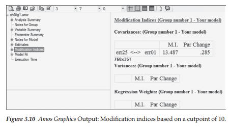
As can be seen in Figure 3.10, there was only one MI that had a value greater than 10. It represented a possible covariance between the error variances related to the indicator variables of SDQ2N25 and SDQ2N01. The MI is shown to be 13.487 and the EPC value to be .285. Interpreted broadly, the MI value suggests that if this parameter were to be freely estimated in a subsequent analysis, the overall chi-square value would drop by approximately 13.487 and the estimated error covariance would take on an approximate value of .285. In essence, this change would not have made any substantial difference to the model fit at all. However, more details regarding the impact of MIs in decisions of whether or not to modify a model will be presented in the next chapter, as well as all remaining chapters.

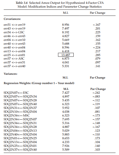
For purposes of comparison, let’s look now at the output file you would have received had the MI cutpoint been left at the Amos default value of 4. As you will note, this information, presented in Table 3.6, contains MIs and EPC values related to error covariances and factor loadings (i.e., the regression weights). Recall that the only model parameters for which the MIs are applicable are those that were fixed to a value of 0.0. Thus, no values appear under the heading Variances as all parameters representing variances (factors and measurement errors) were freely estimated.

In reviewing the parameters in the Covariance section, the only ones that make any substantive sense are those representing error covariances. In this regard, only the parameter representing a covariance between err25 and err01, as noted in Figure 3.9, would appear to be of any inter­est. Nonetheless, as noted above, an MI value of this size (13.487), with an EPC value of .285, particularly as these values relate to an error covari­ance, can be considered of little concern. Turning to the Regression weights, I consider only two to make any substantive sense; these are SDQ2N07 ^ ESC, and SDQ2N34 ^ MSC. Both parameters represent cross-loadings (i.e., secondary loadings). Here again, however, the MIs, and their associated EPC values, are not worthy of inclusion in a subsequently specified model.

Residuals. Recall that the essence of SEM is to determine the fit between the restricted covariance matrix [1(9)], implied by the hypoth­esized model, and the sample covariance matrix (S); any discrepancy between the two is captured by the residual covariance matrix. Each elem­ent in this residual matrix, then, represents the discrepancy between the covariances in 1(9) and those in S [i.e., 1(9) – S]; that is to say, there is one residual for each pair of observed variables (Joreskog, 1993). In the case of our hypothesized model, for example, the residual matrix would contain [(16 x 17)/2] = 136 elements. It may be worth noting that, as in conventional regression analysis, the residuals are not independent of one another. Thus, any attempts to test them (in the strict statistical sense) would be inappropriate. In essence, only their magnitude is of interest in alerting the researcher to possible areas of model misfit.

The matrices of both unstandardized and standardized residuals are available for inclusion in Amos output simply by checking off the Residuals option in the Analysis Properties dialog box (see Figure 3.8).

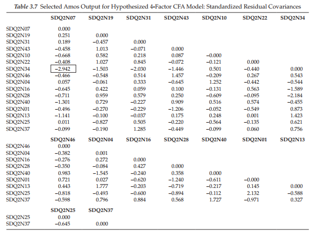
However, because the fitted residuals are dependent on the unit of meas­urement of the observed variables, they can be difficult to interpret and thus their standardized values are typically examined. As such, only the latter are presented in Table 3.7. Standardized residuals are fitted residuals divided by their asymptotically (large sample) standard errors (Joreskog & Sorbom, 1993). As such, they are analogous to Z-scores and are therefore the easier of the two sets of residual values to interpret. In essence, they represent estimates of the number of standard deviations the observed residuals are from the zero residuals that would exist if model fit were perfect [i.e., Σ(θ) – S=0.0]. Values >2.58 are considered to be large (Joreskog & Sorbom, 1993). In examining the standardized residual values presented in Table 3.7, we observe only one that exceeds the cutpoint of 2.58. As such, the standardized residual value of -2.942 reflects on the covariance between the observed variables SDQ2N07 and SDQ2N34. Thus, we can conclude that the only statistically signifi­cant discrepancy of note here lies with the covariance between the two item pairs.

Of prime importance in determining whether or not to include add­itional parameters in a model is the extent to which (a) they are substan­tively meaningful, (b) the existing model exhibits adequate fit, and (c) the EPC value is substantial. Superimposed on this decision is the ever-constant need for scientific parsimony. Because model respecification is commonly conducted in SEM in general, as well as in several applications highlighted in this book, I consider it important to provide you with a brief overview of the various issues related to these post hoc analyses.

5. Post Hoc Analyses

In the application of SEM in testing for the validity of various hypoth­esized models, the researcher will be faced, at some point, with the deci­sion of whether or not to respecify and reestimate the model. If he or she elects to follow this route, it is important to realize that analyses then become framed within an exploratory, rather than a confirmatory mode. In other words, once a hypothesized CFA model, for example, has been rejected, this spells the end of the confirmatory factor analytic approach, in its truest sense. Although CFA procedures continue to be used in any respecification and reestimation of the model, these analyses would then be considered to be exploratory in the sense that they focus on the detec­tion of misfitting parameters in the originally hypothesized model. Such post hoc analyses are conventionally termed “specification searches” (see MacCallum, 1986). (The issue of post hoc model fitting is addressed fur­ther in Chapter 9 in the section dealing with cross-validation.)

The ultimate decision underscoring whether or not to proceed with a specification search is twofold. First and foremost, the researcher must determine whether the estimation of the targeted parameter is substan­tively meaningful. If, indeed, it makes no sound substantive sense to free up the parameter exhibiting the largest MI, then one may wish to consider the parameter having the next largest MI value (Joreskog, 1993). Second, one needs to consider whether or not the respecified model would lead to an overfitted model. The issue here is tied to the idea of knowing when to stop fitting the model, or as Wheaton (1987, p. 123) phrased the prob­lem, “knowing… how much fit is enough without being too much fit.” In general, overfitting a model involves the specification of additional parameters in the model after having determined a criterion that reflects a minimally adequate fit. For example, an overfitted model can result from the inclusion of additional parameters that (a) are “fragile” in the sense of representing weak effects that are not likely replicable, (b) lead to a sig­nificant inflation of standard errors, and (c) influence primary parameters in the model, albeit their own substantive meaningfulness is somewhat equivocal (Wheaton, 1987). Although correlated errors often fall into this latter category,⁹ there are many situations—particularly with respect to social psychological research, where these parameters can make strong substantive sense and therefore should be included in the model (Joreskog & Sorbom, 1993).

Having laboriously worked our way through the process involved in evaluating the fit of a hypothesized model, what can we conclude regard­ing the CFA model under scrutiny in the present chapter? In answering this question, we must necessarily pool all the information gleaned from our study of the Amos output. Taking into account (a) the feasibility and stat­istical significance of all parameter estimates, (b) the substantially good fit of the model, with particular reference to the CFI (.962) and RMSEA (.048) values, and (c) the lack of any substantial evidence of model misfit, I con­clude that any further incorporation of parameters into the model would result in an overfitted model. Indeed, MacCallum et al. (1992, p. 501) have cautioned that, “when an initial model fits well, it is probably unwise to modify it to achieve even better fit because modifications may simply be fitting small idiosyncratic characteristics of the sample.” Adhering to this caveat, I conclude that the 4-factor model schematically portrayed in Figure 3.1 represents an adequate description of self-concept structure for grade 7 adolescents.

6. Hypothesis 2: Self-concept is a 2-Factor Structure

The model to be tested here (Model 2) postulates a priori that SC is a 2-factor structure consisting of GSC and ASC. As such, it argues against the viability of subject-specific academic SC factors. As with the 4-factor model, the four GSC measures load onto the GSC factor; in contrast, all other measures load onto the ASC factor. This hypothesized model is rep­resented schematically in Figure 3.11, which serves as the model specifica­tion for Amos Graphics.

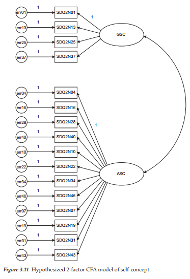
In reviewing the graphical specification of Model 2, two points per­tinent to its modification are of interest. First, while the pattern of factor loadings remains the same for the GSC and ASC measures, it changes for both the ESC and MSC measures in allowing them to load onto the ASC factor. Second, because only one of these eight ASC factor loadings needs to be fixed to 1.0, the two previously constrained parameters (SDQ2N10 ^ ESC; SDQ2N07 ^ MSC) are now freely estimated.

Selected Amos Text Output: Hypothesized 2-Factor Model

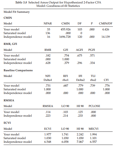
Only the goodness-of-fit statistics are relevant to the present application, and a selected group of these is presented in Table 3.8.

As indicated in the output, the x²(W3) value of 455.926 represents an extremely poor fit to the data, and a substantial decrement from the over­all fit of the 4-factor model (A x²(₅)=297.415). The gain of five degrees of freedom can be explained by the estimation of two fewer factor variances and five fewer factor covariances, albeit the estimation of two additional factor loadings (formerly SDQ2N10 ^ ESC and SDQ2N07 ^ MSC). As expected, all other indices of fit reflect the fact that self-concept structure is not well represented by the hypothesized 2-factor model. In particular, the CFI value of .776 and RMSEA value of .114, together with a PCLOSE value of 0.00 are strongly indicative of inferior goodness-of-fit between the hypothesized 2-factor model and the sample data. Finally, the ECVI value of 1.977, compared with the substantially lower value of 0.888 for the hypothesized 4-factor model again confirms the inferior fit of Model 2.

7. Hypothesis 3: Self-concept is a 1-Factor Structure

Although it now seems obvious that the structure of SC for grade 7 ado­lescents is best represented by a multidimensional SC structure, there are still researchers who contend that SC is a unidimensional construct. Thus, for purposes of completeness, and to address the issue of unidi­mensionality, Byrne and Worth Gavin (1996) proceeded in testing the above hypothesis. However, because the 1-factor model represents a restricted version of the 2-factor model, and thus cannot possibly represent a better-fitting model, in the interest of space, these analyses are not presented here.

In summary, it is evident from these analyses that both the 2-factor and 1-factor models of self-concept represent a misspecification of factor­ial structure for early adolescents. Based on these findings, then, Byrne and Worth Gavin (1996) concluded that SC is a multidimensional con­struct, which in their study comprised the four facets of general, academic, English, and math self-concepts.

8. Modeling with Amos Tables View

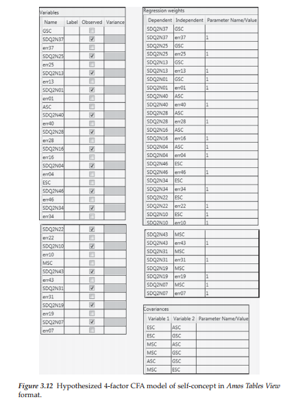
Thus far in this chapter, I have walked you through both the specification and testing of hypothesized models using the Amos Graphics approach. In order to provide you with two perspectives of specifications for the same model, let’s now view the hypothesized 4-factor model (Model 1) within the framework of the Amos Tables View format, which is cap­tured in Figure 3.12. Turning first to the Variables table, you will read­ily note that the only boxes checked are those associated with an item as they represent the only observed variables in the data. In contrast, the constructs of GSC, ASC, ESC, and MSC as latent factors, together with the error terms, represent unobserved variables. Looking next at the Regression weights table, we see a “1” associated with each of the error variances. As you know from Chapter 2, this value of 1.00 indi­cates that the regression path linking the error term with its associated observed variable (the item) is fixed to a value of 1.00 and is therefore not estimated. Finally, the Covariances table reveals that the four factors are hypothesized to covary with one another.

In this first application, testing of the models was fairly straightfor­ward and lacked any additional complexity as a result of the analyses. As a consequence, I was able to present the entire set of Tables in Figure 3.12. However, in the chapters that follow, the models become increasingly complex and thus, due to limitations of space in the writing of a book such as this one, some portions of the Tables View output may need to be eliminated as I zero-in on particular areas of interest. Nevertheless, given that you have full access to the datasets used in this book, I urge you to conduct the same analyses, at which time you will be able to view the entire output.

Source: Byrne Barbara M. (2016), Structural Equation Modeling with Amos: Basic Concepts, Applications, and Programming, Routledge; 3rd edition.