Using the Amos Program

1. Key Concepts

• Building SEM models using Amos Graphics
• Building SEM models using Amos Tables View
• Corollary associated with single variable estimation
• Concept of model (or statistical) identification
• Computing the number of degrees of freedom
• Distinctions between first- and second-order CFA models
• Changing Amos default color for constructed models

The program name, Amos, is actually an acronym for “Analysis of Moment Structures” or, in other words, the analysis of mean and covariance struc­tures, the essence of SEM analyses. From Chapters 3 through 13, I walk you through use of the Amos program in the specification, testing, and interpretation of program output pertinent to a variety of confirmatory factor analytic (CFA) and path analytic models. However, before you can use any program in testing SEM models, it is essential that you first have a solid understanding of how to specify the model under test. In this regard, Amos differs from other SEM programs in that it provides you with a choice of four ways to specify models (described below). Only the graph­ical and recently developed tabular approaches will be illustrated through­out this volume. Based on a walk-through of three basic categories of SEM models, the intent of this chapter is to prepare you for the applications that follow by providing you with the necessary knowledge and technical skills needed in using these two approaches to model specification.

An interesting aspect of Amos is that, although developed within the Microsoft Windows interface and thus commonly considered to represent only a graphical approach to SEM, the program actually allows you to choose from four different modes of model specification. Using the Amos Graphics approach, you first build the model of interest and then work directly from this model in the conduct of various analyses. However, rec­ognizing the fact that not everyone likes to work with graphics, Arbuckle (2012) recently (i.e., Version 21) introduced a Tables View¹ alternative. In lieu of building the model to be tested graphically, this option enables you to create exactly the same model, albeit using a spreadsheet approach. As such, all parameters of the model are listed in one of three or more tables each of which represents a common set of model components. Given that the Graphics and Tables View approaches to model specification represent two sides of the same coin, Arbuckle (2012) cleverly devised a tab on the Amos Graphics workspace that enables you to switch from one view to the other. For example, if you built the model graphically, then clicking on this tab would present you with the same model in Tables View for­mat. Likewise, if you structured the model via Tables View, then a sche­matic representation of the equivalent model is just a click away. Lastly, the remaining two approaches, Amos VB.NET and Amos C#, enable you to work directly from equation statements. Regardless of which type of model specification you choose, all options related to the analyses are available from drop-down menus, and all estimates derived from the ana­lyses can be presented in text format. In addition, however, Amos Graphics allows for the estimates to be displayed graphically in a path diagram.

The choice of which Amos method to use for model specification is purely arbitrary and really boils down to how comfortable you feel in working within either a graphical or table interface versus a more trad­itional programming interface. However, given the overwhelming popu­larity of the Amos Graphics approach to model specification by Amos users, together with the issue of space limitations, applications based on Amos VB.NET and/or Amos C# are not included in this volume. Nonetheless, for those who may be interested in using one or both of these approaches to model specification, detailed information can be accessed through the Amos Online Help option and many model examples can be found in the Amos User’s Guide (Arbuckle, 2015).

Throughout this third edition of the book, I focus primarily on the Amos Graphical approach to SEM, but include the equivalent Tables View representation of each model under study. Without a doubt, for those of you who enjoy working with draw programs, rest assured you will love working with Amos Graphics! All drawing tools have been carefully designed with SEM conventions in mind—and there is a wide array of them from which to choose. With a simple click of either the left or right mouse buttons, you will be amazed at how quickly you can build and spe­cify an SEM model, run analyses in testing the model, and/or formulate a publication-quality path diagram.

In this chapter only, I walk you through the steps involved in the building of three example models based on Amos Graphics. In addition, given the newness of the Tables View format, I walk you through the same model specification process, albeit pertinent to the Example 1 only, using this table format option. So, let’s turn our attention first to a review of the various components and characteristics of Amos Graphics as they relate to the specification of three basic models—a first-order CFA model (Model 1), a second-order CFA model (Model 2), and a full SEM model (Model 3).

2. Model Specification Using Amos Graphics (Example 1)

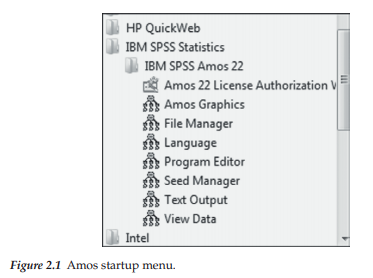
To initiate Amos Graphics, you will need, first, to follow the usual Windows procedure as follows: Click on Start ^ All Programs ^ IBM SPSS Statistics ^ IBM SPSS Amos 23. As shown here, all work in this edition is based on Amos Version 23. Clicking on IBM SPSS Amos 23 pre­sents the complete Amos selection listing. As shown in Figure 2.1, it is possible to access various files pertinent to previous work (e.g., data and model files, as well as other aspects of modeling in Amos). Initially, you will want to click on Amos Graphics. Alternatively, you can always place the Amos Graphics icon on your desktop.

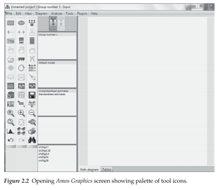
Once you click on Amos Graphics, you will see the opening screen and toolbox shown in Figure 2.2. On the far right of this screen you will see a blank rectangle; this space provides for the drawing of your path diagram. The large highlighted icon at the top of the center section of the screen, when activated, presents you with a view of the input path diagram (i.e., the model specification). The companion icon to the right of the first one allows you to view the output path diagram; that is, the path diagram with the parameter estimates included. Of course, given that we have not yet conducted any analyses, this output icon is grayed out and not highlighted.

3. Amos Modeling Tools

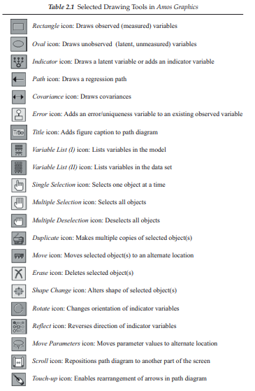
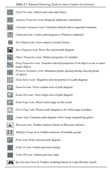
Amos provides you with all the tools that you will ever need in creating and working with SEM path diagrams. Each tool is represented by an icon (or button) and performs one particular function; there are 42 icons from which to choose. As shown in Figure 2.2, the toolbox containing each of these icons is located on the far left of the palette. A brief description of each icon is presented in Table 2.1.

In reviewing Table 2.1, you will note that, although the majority of the icons are associated with individual components of the path dia­gram (e.g., |o]0), or with the path diagram as a whole (e.g., HU |Q]), oth­ers relate either to the data (e.g., H) or to the analyses (e.g., g]). Don’t worry about trying to remember this smorgasbord of tools, as simply holding the mouse pointer stationary over an icon is enough to trigger the pop-up label that identifies its function. As you begin working with Amos Graphics in drawing a model, you will find two tools, in particular, the Indicator icon [W] and the Error icon [g], to be worth their weight in gold! Both of these icons reduce, tremendously, the tedium of trying to align all multiple indicator variables, together with their related error variables in an effort to produce an aesthetically pleasing diagram. As a consequence, it is now possible to structure a path diagram in just a matter of minutes.

Now that you have had a chance to peruse the working tools of Amos Graphics, let’s move on to their actual use in formulating a path diagram. For your first experience in using this graphical interface, we’ll reconstruct the hypothesized CFA model shown in Figure 2.3.

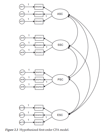
4. The Hypothesized Model

The CFA structure in Figure 2.3 comprises four self-concept (SC) factors—academic SC (ASC), social SC (SSC), physical SC (PSC), and emo­tional SC (ESC). Each SC factor is measured by three observed variables, the reliability of which is influenced by random measurement error, as indicated by the associated error term. Each of these observed variables is regressed onto its respective factor. Finally, the four factors are shown to be intercorrelated.

5. Drawing the Path Diagram

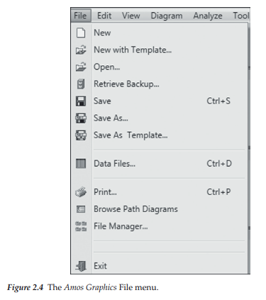
To initiate the drawing of a new model, click on File shown at the top of the opening Amos screen and then select New from the drop-down menu. Although the File drop-down menu is typical of most Windows programs, I include it here in Figure 2.4 in the interest of completeness.

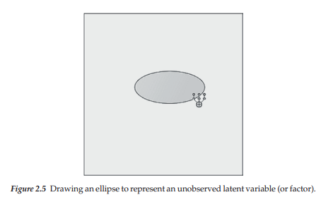
Now, we’re ready to draw our path diagram. The first tool you will want to use is, what I call, the “million dollar” (Indicator) icon (see Table 2.1) because it performs several functions. Click on this icon to acti­vate it and then, with the cursor in the blank drawing space provided, hold down the left mouse button and draw an ellipse by dragging it slightly to create an ellipse shape.² If you prefer your factor model to show the factors as circles, rather than ellipses, just don’t perform the dragging action. When working with the icons, you need to release the mouse button after you have finished working with a particular func­tion. Figure 2.5 illustrates the completed ellipse shape with the Indicator icon [*g] still activated. Of course, you could also have activated the Draw Unobserved Variables icon [£] and achieved the same result.

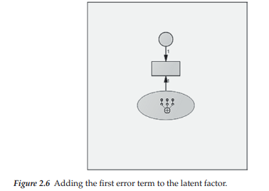
Now that we have the ellipse representing the first latent factor, the next step is to add the indicator variables. To do so, we click on the Indicator icon, after which the mouse pointer changes to resem­ble the Indicator icon. Now, move the Indicator icon image to the center of the ellipse at which time its outer rim becomes highlighted in red. Next, click on the unobserved variable. In viewing Figure 2.6, you will see that this action produces a rectangle (representing a single observed variable), an arrow pointing from the latent factor to the observed vari­able (representing a regression path), and a small circle with an arrow pointing toward the observed variable (representing a measurement error term).³ Again, you will see that the Indicator icon, when activated, appears in the center of the ellipse. This, of course, occurs because that’s where the cursor is pointing.

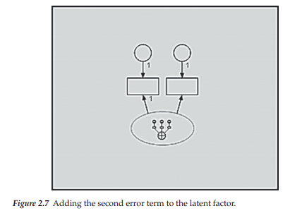
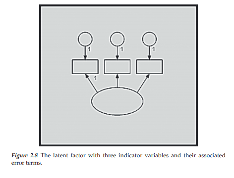
Note, however, that the hypothesized model (see Figure 2.3) we are endeavoring to structure schematically shows each of its latent factors to have three indicator variables, rather than only one. These additional indicators are easily added to the diagram by two simple clicks of the left mouse button while the Indicator icon is activated. In other words, with this icon activated, each time that the left mouse button is clicked, Amos Graphics will produce an additional indicator variable, each with its asso­ciated error term. Figures 2.7 and 2.8 show the results of having made one and two additional clicks, respectively, to the left mouse button.

In reviewing the hypothesized model again, we note that the three indicator variables for each latent factor are oriented to the left of the ellipse rather than to the top, as is currently the case in our diagram here. This task is easily accomplished by means of rotation. One very simple way of accomplishing this reorientation, is to click the right mouse button while the Indicator icon is activated. Figure 2.9 illustrates the outcome of this clicking action.

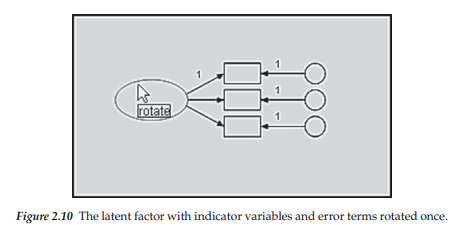
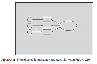
As you can see from the dialog box, there are a variety of options related to this path diagram from which you can choose. At this time, however, we are only interested in the Rotate option. Moving down the menu and clicking with the left mouse button on Rotate will activate the Rotate function and assign the related label to the cursor. When the cursor is moved to the center of the oval and the left mouse button clicked, the three indicator variables, in combination with their error terms and links to the underlying factor, will move 45 degrees clockwise as illustrated in Figure 2.10; two additional clicks will produce the desired orientation shown in Figure 2.11. Alternatively, we could have activated the Rotate icon [G] and then clicked on the ellipse to obtain the same effect.

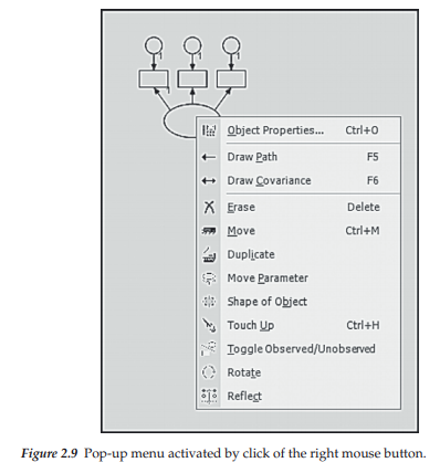
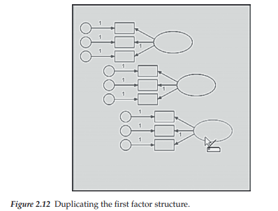
Now that we have a one-factor structure completed, it becomes a simple task of duplicating this configuration in order to add three addi­tional ones to the model. However, before we can duplicate, we must first group all components of this structure so that they operate as a sin­gle unit. This is easily accomplished by clicking on the Multiple Selection icon 0], after which you will observe that the outline of all factor struc­ture components is now highlighted in blue, thereby indicating that they now operate as a unit. As with other drawing tasks in Amos, duplication of this structure can be accomplished either by clicking on the Duplicate icon [§], or by right-clicking on the model and activating the menu as shown in Figure 2.9. In both cases, you will see that with each click and drag of the left mouse button, the cursor takes on the form of a pho­tocopier and generates one copy of the factor structure. This action is illustrated in Figure 2.12.

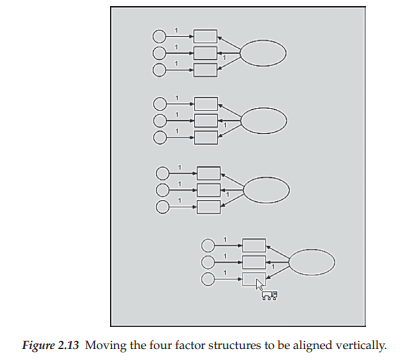
Once you have the number of copies that you need, it’s just a matter of dragging each duplicated structure into position. Figure 2.13 illustrates the four factor structures lined up vertically to replicate the hypothesized CFA model. Note the insert of the Move icon [™j in this figure. It is used to reposition objects from one location to another. In the present case, it was used to move the four duplicated factor structures such that they were aligned vertically. In composing your own SEM diagrams, you may wish to move an entire path diagram for better placement on a page. This rea­lignment is made possible with the Move Icon, but don’t forget to activate the Select All icon illustrated first.⁴

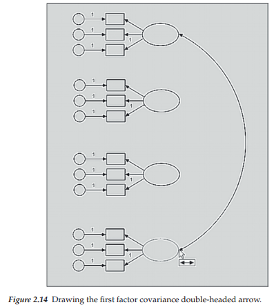
Now we need to add the factor covariances to our path diagram. Illustrated in Figure 2.14 is the addition of a covariance between the first and fourth factors; these double-headed arrows are drawn by clicking on the Covariance icon 0. Once this button has been activated, you then click on one object (in this case, the first latent factor), and drag the arrow to the second object of interest (in this case, the fourth latent factor). The process is then repeated for each of the remaining specified covariances. Yes, gone are the days of spending endless hours trying to draw multi­ple arrows that look at least somewhat similar in their curvature! Thanks to Amos Graphics, these double-headed arrows are drawn perfectly every single time.

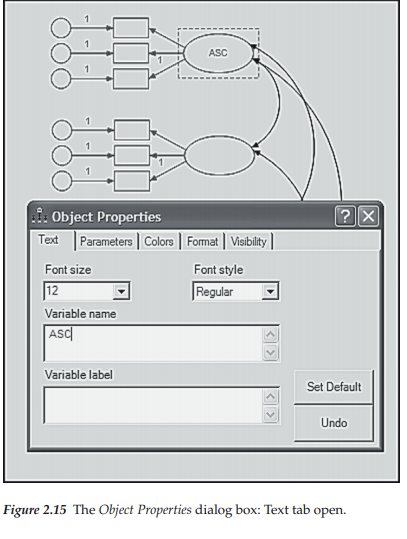
At this point, our path diagram, structurally speaking, is complete; all that is left to be done is to label each of the variables. If you look back at Figure 2.9, in which the mouse right-click menu is displayed, you will see a selection termed Object Properties at the top of the menu. This is the option you need in order to add text to a path diagram. To initiate this pro­cess, point the cursor at the object in need of the added text, right-click to bring up the View menu, and finally, left-click on Object Properties, which activates the dialog box shown in Figure 2.15. Of the five different tabs at the top of the dialog box, we select the Text tab, which then enables us to select a font size and style specific to the variable name to be entered. For purposes of illustration, I have simply entered the label for the first latent variable (ASC) and selected a font size of 12 with regular font style. All remaining labeling was completed in the same manner. Alternatively, you can display the list of variables in the data and then drag each variable to its respective rectangle.

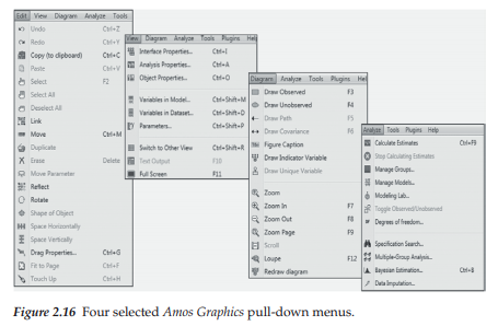
The path diagram related to the hypothesized CFA model is now com­plete. However, before leaving Amos Graphics, I wish to show you the con­tents of four pull-down menus made available to you on your drawing screen. (For a review of a possible eight menus, see Figure 2.2.) The first and third drop-down menus (Edit; Diagram) shown in Figure 2.16 relate in some way to the construction of path diagrams. In reviewing these two menus, you will quickly see that they serve as alternatives to the use of drawing tools, some of which I have just demonstrated in the reconstruction of Figure 2.3. Thus, for those of you who may prefer to work with pull-down menus, rather than with drawing tool buttons, Amos Graphics provides you with this option. As its name implies, the View menu allows you to per­use various features associated with the variables and/or parameters in the path diagram. An important addition to this drop-down menu is the “Switch to Other View” option which, as noted earlier, was implemented in Version 21. As noted earlier regarding the tab on the Amos Graphics work­space, this option enables you to switch from a graphical view of a model to a parallel table view and vice versa. Finally, from the Analyze menu, you can calculate estimates (i.e., execute a job), manage groups and/or models, and conduct multiple group analyses as well as other types of analyses.

By now, you should have a fairly good understanding of how Amos Graphics works. Of course, because learning comes from doing, you will most assuredly want to practice some of the techniques illustrated here on your own.

For those of you who may still feel a little uncomfortable in work­ing with the Amos Graphical approach to model building, I now walk you through the basic steps involved in specification of the same 4-factor model using the Tables View approach.

5. Model Specification Using Amos Tables View (Example 1)

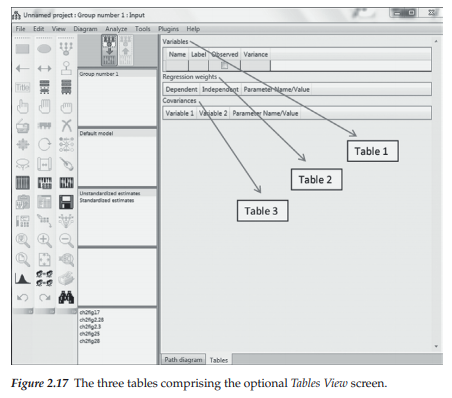
As noted earlier, and as seen in Figure 2.2, the tab appearing at the base of the Amos work space enables you to build a model either as a path diagram using the graphical interface, or as a set of tables using the Tables View interface. Clicking on the “Path diagram” tab results in the blank worksheet shown in Figure 2.2.⁵ Alternatively, clicking on the “Tables” tab results in the work space shown in Figure 2.17. Closer examination of this space reveals three tables which, when used in combination, provide all the information needed in the specification of a CFA model. The first of these tables, labeled Variables, allows for identification of which vari­ables are observed and which are not observed (i.e., latent). The next table, labeled Regression weights, provides information on which parameters (i.e., factor loadings and error variance terms) are fixed to 1.0 for purposes of model (or statistical) identification, a topic to be discussed immediately following this introduction to the Tables View interface. Finally, the third table, labeled Covariances, enables specification of which latent factors are hypothesized to covary with one another.

Let’s now walk through the process of specifying the 4-factor CFA model schematically displayed in Figure 2.3 using the Tables View approach.^6,7 Shown in Figure 2.18 are the three tables noted above, albeit with all specification information inserted in the appropriate cells. As such, the model, as specified in path analysis mode (Figure 2.3), is equiva­lent to Tables View mode (Figure 2.18). As I now explain the content of all table cells, I highly recommend that you have both Figures 2.3 and 2.18 in full view in order that you will fully comprehend the extent to which they are comparable to one another.

Let’s focus first on the first three lines of the Variables table in Figure 2.18. In the initial row, we see that the latent variable (ASC) has been entered, followed next by the first indicator variable (SDQASC1) associated with ASC, and finally, the error variance parameter associated with SDQASC1 (err1). Of these three parameters, only the SDQASC1 variable is observed

and, thus, the only one for which there is a checkmark appearing in the Observed column. The next four rows provide the same information, albeit related to the two additional indicator variables associated with ASC. Thus, the first seven rows of cells are pertinent only to Factor 1 of this model. Likewise, the next three sets of seven rows provide specification information for Factor 2 (SSC), Factor 3 (PSC, and Factor 4 (ESC).

Turning next to the Regression weights table, we see three columns labeled as “Dependent,” “Independent,” and “Parameter Name/Value.” In the first column, only the observed variables are listed, with each appearing on two consecutive rows. In all CFA models, the observed variables are always dependent variables in the model because, as shown in Figure 2.3, they have two sets of arrows (representing regression paths) pointing at them; the single-headed arrow leading from the latent variable to the observed variable represents the factor loading, and the one leading from the error term represents the impact of measurement error on the observed variable. Thus, for each line showing the same observed variable (e.g., SDQASC1), in column 2 you will see the two parameters on which it is regressed (e.g., ASC and errorl). This matching pattern is consistent for all observed vari­ables in the model. Finally, in column 3, you will see a specification of “1”, but only for some of the entries in column 2. The reason for these entries of “1” is twofold. First, in a review of Figure 2.3, you will note that all regres­sion paths leading from the error variances to the observed (or indicator) variables are shown with the numeral “1” above it, thereby signaling that these parameters are not estimated but, rather, are fixed to a value of “1”.

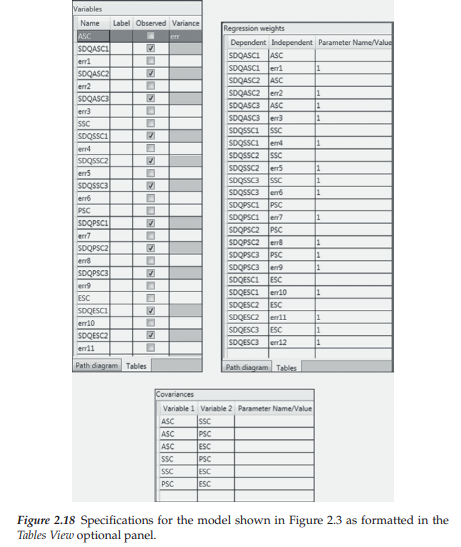
This specification addresses an important corollary in the modeling of sin­gle variables in SEM—you can estimate either the variance or the regression path, but you cannot estimate both. Because the error variance associated with each observed variable is of critical importance, its related error regres­sion path is constrained to a fixed value of “1”. For this reason, then, error regression paths, by default, are automatically fixed to “1” in all SEM pro­grams and this is the case here with respect to Amos. Thus, in reviewing these values in Column 3, you will see that the value of “1” is associated with all of the error terms. Second, turning again to Figure 2.3, you will note that the third indicator variable associated with each factor (e.g., SDQASC3 with ASC) is also fixed to “1”. Correspondingly, this value appears on the sixth line of the third column of the Regression weights table in Figure 2.18 as it relates to the same indicator/latent variable pairing; likewise for the three remaining factor loadings that have been constrained to “1” (SDQSSC3/ SSC; SDQPSC3/PSC; SDQESC/ESC). These fixed values address the issue of model (or statistical) identification, a topic to which we turn shortly.

Finally, in reviewing Figure 2.3 once again, you will note that the four latent factors are hypothesized to be intercorrelated as indicated by the double-headed arrows joining them. Turning to the table in Figure 2.18, it is easy to see that these same latent variable links are specified in table form via Columns 1 and 2.

In specifying a model using Tables View, I wish to pass along a few hints that I hope you will find helpful:

• The sudden appearance of a red circle with an exclamation mark in its center serves as notification that something is wrong in a par­ticular row. Running the mouse over this circle will yield the error message; typically, the problem is that you have inserted the same information in one of the other cells.
• I purposefully entered information into the cells consistent with the labeling of the model in Figure 2.3 in order to keep things simple here. That is, I started at the top of the model with ASC and its related indicator variables. However, this type of ordering is not necessary. Rather, as long as you keep the same groupings together (e.g., ASC and its indicator variables), the order in which they are entered doesn’t matter (J. Arbuckle, personal communication, February 4,2014).
• It can be difficult to alter the ordering of the regression weights once they have been entered. One workable solution is to completely delete the originally entered regression weight and then enter it again, albeit with the new regression weight value. Important to know here, how­ever, is that the new weight will be added at the bottom of the list and the initial value should automatically be deleted from program memory (J. Arbuckle, personal communication, February 5, 2014).

As noted at the beginning of this journey into building models via the Tables View option, a single click of the dual Path diagram/Tables tab at the bottom of the Amos work space (see Figure 2.2 and 2.17) enables the user to easily switch between the two options. Given that we have now com­pleted our specification of the CFA shown in Figure 2.3, no doubt you are expecting to see an exact replication of this figure once you click on the Path diagram tab. Thus, I’m sure it will be with some degree of shock that you view the model as completed in table format! Indeed, Figure 2.19 reveals exactly what you will see. Although the various components of the model look to be very random, this is not exactly the case. It’s just that in the process of adding each of the components to the model, Amos tries to prevent the circles and squares from overlapping, as well as to keep the arrows fairly short.

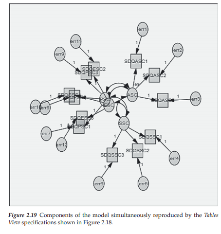
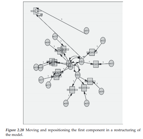
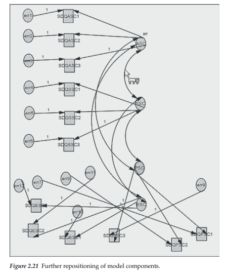
It is important to note that there is no need to reconstruct these elem­ents to resemble the model in Figure 2.3. Even though the assemblage might look like a complete mess, rest assured that Amos knows all com­ponents of the model, as well as the specification of their related parame­ters. Thus, despite the rather disheveled-looking figure that you find upon completing the tables, all subsequent analyses remain the same as if you had built the model graphically. However, should you prefer to rearrange the components into the appropriate model, you can easily accomplish this task by working with selected draw tools from the toolbox. Likely the most valuable tool for this operation is the Move icon, introduced earlier in this chapter. Here, Figure 2.20 illustrates the beginning of this reconstruc­tion process whereby the first indicator variable (SDQASC1) has been selected and moved to the top of the work page. Following the moving of several more of the indicator variables, latent factors, and single-headed and double-headed arrows, Figure 2.21 enables you to see the gradual for­mation of our 4-factor model of interest.

Now that you have been introduced to use of both the Amos Graphics and Tables View approaches to model specification, let’s move forward and examine our example Model 1 (see Figure 2.3) in more detail. We begin by studying the model’s basic components, default specification of particular parameters by the Amos program, and the critically important concept of model (or statistical) identification.

6. Understanding the Basic Components of Model 1

Recall from Chapter 1 that the key parameters to be estimated in a CFA model are the regression coefficients (i.e., factor loadings), the latent factor and error variances, and in some models (as is the case with Figure 2.3) the factor covariances. Given that the latent and observed variables are specified in the model in Amos Graphics (and in its Tables View alternative), the program automatically estimates the factor and error variances. In other words, variances associated with these specified variables are freely estimated by default. However, defaults related to parameter covariances, using Amos, are governed by the WYSIWYG rule—What You See Is What You Get. That is, if a covariance path is not included in the path diagram (or the matching table format), then this parameter will not be estimated (by default); if it is included, then its value will be estimated.

One extremely important caveat in working with structural equation models is to always tally the number of parameters in the model being estimated prior to running the analyses. This information is critical to your knowledge of whether or not the model that you are testing is statistically identified. Thus, as a prerequisite to the discussion of identification, let’s count the number of parameters to be estimated for the model portrayed in Figure 2.3. From a review of the figure, we can ascertain that there are 12 regression coefficients (factor loadings), 16 variances (12 error variances and 4 factor variances), and 6 factor covariances. The 1s assigned to one of each set of regression path parameters represent a fixed value of 1.00; as such, these parameters are not estimated. In total, then, there are 30 parameters to be estimated for the CFA model depicted in Figure 2.3. Let’s now turn to a brief discussion of the critically important concept of model (or statistical) identification.

7. The Concept of Model Identification

Model identification is a complex topic that is difficult to explain in non­technical terms. Although a thorough explanation of the identification principle exceeds the scope of the present book, it is not critical to the reader’s understanding and use of Amos in the conduct of SEM analyses. Nonetheless, because some insight into the general concept of the iden­tification issue will undoubtedly help you to better understand why, for example, particular parameters are specified as having values fixed to say, 1.00, I attempt now to give you a brief, nonmathematical explanation of the basic idea underlying this concept. Essentially, I address only the so-called “t-rule”, one of several tests associated with identification. I encourage you to consult the following texts for more comprehensive treatments of the topic: Bollen, 1989a; Kline, 2011; Long, 1983a, 1983b; Saris & Stronkhorst, 1984. I also highly recommend two book chapters having very clear and readable descriptions of the identification issue (Kenny & Milan, 2012; MacCallum, 1995), as well as an article addressing the related underlying assumptions (see Hayashi & Marcoulides, 2006).

In broad terms, the issue of identification focuses on whether or not there is a unique set of parameters consistent with the data. This question bears directly on the transposition of the variance-covariance matrix of observed variables (the data) into the structural parameters of the model under study. If a unique solution for the values of the structural param­eters can be found, the model is considered to be identified. As a con­sequence, the parameters are considered to be estimable and the model therefore testable. If, on the other hand, a model cannot be identified, it indicates that the parameters are subject to arbitrariness, thereby imply­ing that different parameter values define the same model; such being the case, attainment of consistent estimates for all parameters is not possible and, thus, the model cannot be evaluated empirically.

By way of a simple example, the process would be conceptually akin to trying to determine unique values for X and Y, when the only informa­tion you have is that X + Y = 15. Put another way, suppose that I ask you what two numbers add up to 15? You could say, for example, 10 + 5; 14 + 1; 8 + 7 and so on. In this instance, given that there are many ways by which you could attain the summation of 15, there is clearly no unique answer to the question. However, let’s say I ask you the same question but, instead, add that one of the numbers is 8; now you know exactly which number to select and therefore have a unique answer. Thus, by simply fixing the value of one number in the equation, you can immediately identify the missing number. Generalizing this simple example to SEM (also referred to as the analysis of covariance structures), the model identification issue focuses on the extent to which a unique set of values can be inferred for the unknown parameters from a given covariance matrix of analyzed variables that is reproduced by the model. Hopefully, this example also explains the basic rationale underlying the fixed value of 1.00 assigned to certain parameters in our specification of Model 1 in this chapter.

Structural models may be just-identified, overidentified, or underiden­tified. A just-identified model is one in which there is a one-to-one cor­respondence between the data and the structural parameters. That is to say, the number of data variances and covariances equals the number of parameters to be estimated. However, despite the capability of the model to yield a unique solution for all parameters, the just-identified model is not scientifically interesting because it has no degrees of freedom and therefore can never be rejected. An overidentified model is one in which the number of estimable parameters is less than the number of data points (i.e., variances and covariances of the observed variables). This situation

results in positive degrees of freedom that allow for rejection of the model, thereby rendering it of scientific use. The aim in SEM, then, is to specify a model such that it meets the criterion of overidentification. Finally, an underidentified model is one in which the number of parameters to be estimated exceeds the number of variances and covariances (i.e., data points). As such, the model contains insufficient information (from the input data) for the purpose of attaining a determinate solution of param­eter estimation; that is, an infinite number of solutions are possible for an underidentified model.

Reviewing the CFA model in Figure 2.3, let’s now determine how many data points we have to work with (i.e., how much information do we have with respect to our data?). As noted above, these constitute the variances and covariances of the observed variables; with p variables, there are p(p + 1)/2 such elements. Given that there are 12 observed vari­ables, this means that we have 12(12 + 1)/2 = 78 data points. Prior to this discussion of identification, we determined a total of 30 unknown param­eters. Thus, with 78 data points and 30 parameters to be estimated, we have an overidentified model with 48 degrees of freedom.

However, it is important to note that the specification of an overiden­tified model is a necessary, but not a sufficient condition to resolve the identification problem. Indeed, the imposition of constraints on particular parameters can sometimes be beneficial in helping the researcher to attain an overidentified model. An example of such a constraint is illustrated in Chapter 5 with the application of a second-order CFA model.

Linked to the issue of identification is the requirement that every latent variable have its scale determined. This constraint arises because these variables are unobserved and therefore have no definite metric scale; it can be accomplished in one of two ways. The first approach is tied to specification of the measurement model, whereby the unmeasured latent variable is mapped onto its related observed indicator variable. This scal­ing requisite is satisfied by constraining to some nonzero value (typically 1.0), one factor loading parameter in each congeneric⁸ set of loadings. This constraint holds for both independent and dependent latent variables. In reviewing Figure 2.3, then, this means that for one of the three regression paths leading from each SC factor to a set of observed indicators, some fixed value should be specified; this fixed parameter is termed a reference variable.⁹ With respect to the model in Figure 2.3, for example, the scale has been established by constraining to a value of 1.0 the third parameter in each set of observed variables. Recall that in working through the Amos Graphical specification of Model 1, the program automatically assigned this value when the Indicator Variable icon was activated and used to add the first indicator variable and its error term to the model. Recall also, how­ever, that these values were not added automatically with specification of the model using the table format. It is important to note that although Amos Graphics assigned the value of “1” to the lower regression path of each set, this assignment can be changed simply by clicking on the right mouse button and selecting Object Properties from the pop-up menu. (This modification will be illustrated with the next example.)

With a better idea of important aspects of the specification of a CFA model in general, specification using Amos (either the graphical or table format) in particular, as well as the basic notions associated with model identification, we now continue on our walk through the two remaining models reviewed in this chapter. As with Model 1, we begin by specifying Model 2 using the graphical approach to model specification.

8. Model Specification Using Amos Graphics (Example 2)

In this second example of model specification, we examine the second-order model displayed in Figure 2.22.

The Hypothesized Model

In our previous factor analytic model, we had four factors (ASC, SSC, PSC, ESC) which operated as independent variables; each could be considered to be one level, or one unidirectional arrow away from the observed vari­ables. Such factors are termed first-order factors. However, it may be the case that the theory argues for some higher-level factor that is considered accountable for the lower-order factors. Basically, the number of levels or unidirectional arrows that the higher-order factor is removed from the observed variables determines whether a factor model is considered to be second-order, third-order, or some higher-order. Only a second-order model will be examined here.

Although the model schematically portrayed in Figure 2.22 has essen­tially the same first-order factor structure as the one shown in Figure 2.3, it differs in that a higher-order general self-concept (GSC) factor is hypoth­esized as accounting for, or explaining, all variance and covariance related to the first-order factors. As such, GSC is termed the second-order factor. It is important to take particular note of the fact that GSC does not have its own set of measured indicators; rather it is linked indirectly to those measuring the lower-order factors.

Let’s now take a closer look at the parameters to be estimated for this second-order model (Figure 2.22). First, note the presence of single-headed arrows leading from the second-order factor (GSC) to each of the first-order factors (ASC to ESC). These regression paths represent second-order fac­tor loadings, and all are freely estimated. Recall, however, that for reasons linked to the model identification issue, a constraint must be placed either on one of the regression paths, or on the variance of an independent fac­tor as these parameters cannot be estimated simultaneously. Because the impact of GSC on each of the lower-order SC factors is of primary inter­est in second-order CFA models, the variance of the higher-order factor is typically constrained to equal 1.0, thereby leaving the second-order factor loadings to be freely estimated.

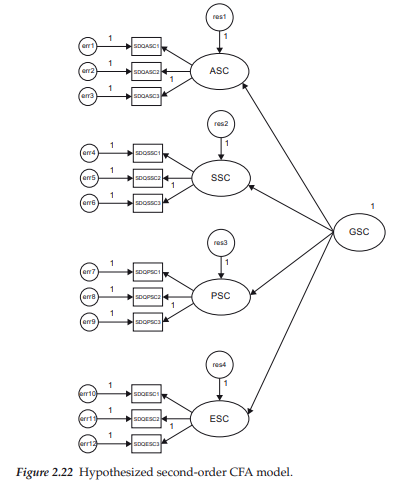
A second aspect of this second-order model that perhaps requires some amplification is the initial appearance of the first-order factors operating as both independent and dependent variables. This situa­tion is not so, however, as variables can serve either as independent or as dependent variables in a model, but not as both.¹⁰ Because the first-order factors function as dependent variables, it then follows that their variances and covariances are no longer estimable parameters in the model; such variation is presumed to be accounted for by the higher-order factor. In comparing Figures 2.3 and 2.22, then, you will note that there are no longer double-headed curved arrows linking the first-order SC factors, indicating that neither the factor covariances nor variances are to be estimated.

Finally, the prediction of each of the first-order factors from the second-order factor is presumed not to be without error. Thus, a residual error term is associated with each of the lower-level factors.

As a first step in determining whether this second-order model is identified we now sum the number of parameters to be estimated; we have 8 first-order regression coefficients, 4 second-order regression coef­ficients, 12 measurement error variances, and 4 residual error terms, mak­ing a total of 28. Given that there are 78 pieces of information in the sample variance-covariance matrix, we conclude that this model is identified with 50 degrees of freedom.

Before leaving this identification issue, however, a word of cau­tion is in order. With complex models in which there may be more than one level of latent variable structures, it is wise to visually check each level separately for evidence that identification has been attained. For example, although we know from our initial CFA model that the first-order level is identified, it is quite possible that the second-order level may indeed be underidentified. Given that the first-order factors function as indicators of (i.e., the input data for) the second-order fac­tor, identification is easy to assess. In the present model, we have four factors, giving us 10 (4 x 5/2) pieces of information from which to formulate the parameters of the higher-order structure. According to the model depicted in Figure 2.22, we wish to estimate 8 parameters (4 regression paths; 4 residual error variances), thus leaving us with 2 degrees of freedom, and an overidentified model. However, suppose that we only had three first-order factors. We would then be left with a just-identified model at the upper level as a consequence of trying to estimate 6 parameters from 6 (3[3 + 1])/2) pieces of information. In order for such a model to be tested, additional constraints would need to be imposed (see, e.g., Chapter 5). Finally, let’s suppose that there were only two first-order factors; we would then have an underidenti­fied model since there would be only three pieces of information, albeit four parameters to be estimated. Although it might still be possible to test such a model, given further restrictions on the model, the researcher would be better advised to reformulate his or her model in light of this problem (see Rindskopf & Rose, 1988).

Drawing the Path Diagram

Now that we have dispensed with the necessary “heavy stuff,” let’s move on to creating the second-order model shown in Figure 2.22, which will serve as the specification input for Amos Graphics. We can make life easy for ourselves here simply by pulling up our first-order model (see Figure 2.3). Because the first-order level of our new model will remain the same as that shown in Figure 2.3, the only thing that needs to be done by way of modification is to remove all the factor covariance arrows. This task, of course, can be accomplished in Amos in one of two ways: either by activating the Erase icon [X] and clicking on each double-headed arrow, or by placing the cursor on each double-headed arrow individually and then right-clicking on the mouse, which produces the menu shown earlier.

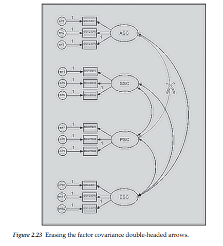
Once you select the Erase option on the menu, the Erase icon will automat­ically activate and the cursor converts to a claw-like X symbol. Simply place the X over the component that you wish to delete and left-click; the targeted component disappears. As illustrated in Figure 2.23, the covari­ance between ASC and SSC has already been deleted with the covariance between ASC and PSC being the next one to be deleted. For both methods of erasure, Amos automatically highlights the selected parameter in red.

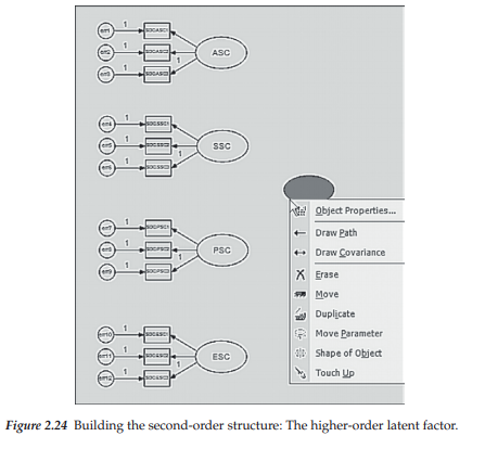
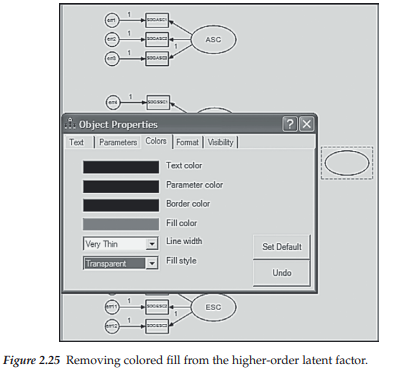
Having removed all the double-headed arrows representing the fac­tor covariances from the model, our next task is to draw the ellipse repre­senting the higher-order factor of GSC. We do this by activating the Draw Unobserved Variable icon [o], which, for me, resulted in an ellipse with solid red fill. However, for publication purposes, you will likely want the ellipse to be clear. To accomplish this, placing the cursor over the upper ellipse and right-clicking on the mouse again will produce a menu from which you select Object Properties. At this point, your model should resemble the one shown in Figure 2.24. Once in this dialog box, click on the Color tab, scroll down to Fill style, and then choose Transparent as illustrated in Figure 2.25. Note that you can elect to set this color option as default by clicking on the Set Default tab to the right.

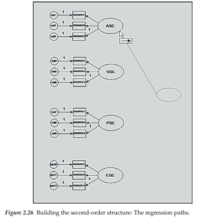
Continuing with our path diagram, we now need to add the second-order factor regression paths. We accomplish this task by first activating the Path icon 0 and then, with the cursor clicked on the central underside of the GSC ellipse, dragging the cursor up to where it touches the central right side of the ASC ellipse. Figure 2.26 illustrates this draw­ing process with respect to the first path; the process is repeated for each of the other three paths.

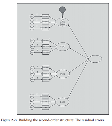
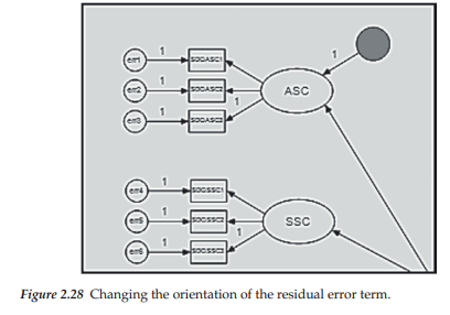
Because each of the first-order factors is now a dependent variable in the model, we need to add the residual error term associated with the prediction of each by the higher-order factor of GSC. To do so, we acti­vate the Error icon [g] and then click with the left mouse button on each of the ellipses representing the first-order factors. Figure 2.27 illustrates implementation of the residual error term for ASC. In this instance, only one click was completed, thereby leaving the residual error term in its current position (note the solid fill as I had not yet set the default for transparent fill). However, if we clicked again with the left mouse button, the error term would move 45 degrees clockwise as shown in Figure 2.28; with each subsequent click, the error term would continue to be moved clockwise in a similar manner.

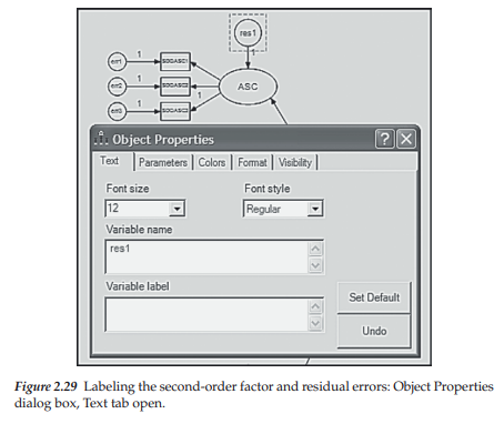
The last task in completing our model is to label the higher-order fac­tor, as well as each of the residual error terms. Recall that this process is accomplished by first placing the cursor on the object of interest (in this case the first residual error term) and then clicking with the right mouse button. This action releases the pop-up menu shown in Figure 2.24 from which we select Object Properties, which, in turn, yields the dialog box dis­played in Figure 2.29. To label the first error term, we again select the Text tab and then add the text, res1; this process is then repeated for each of the remaining residual error terms.

9. Model Specification Using Amos Tables View (Example 2)

Let’s now view specification of this higher-order model from the Tables View perspective as presented in Figure 2.30. Turning first to the Variables table, you will note that, except for the last five rows (denoted by a side bracket), all specifications replicate those reported for the first-order model as shown in Figure 2.18. To fully comprehend the differences between the two model parameterizations, it is best to view both the model (Figure 2.22) and its matching tabled specifications (Figure 2.30) side by side. Note first that the higher-order factor GSC is now included and, in contrast to the other factors, has its variance fixed to a value of 1.00. This specification is then followed by the addition of four residual error terms, given that the four first-order factors are now dependent variables in the model.

Turning to the Regression weights table, you will see the addition of eight parameters, again singled out by a side bracket. Specification of the first-order factors (ASC, SSC, PSC, and ESC) in the first (Dependent) column, together with that of GSC in the second (Independent) column, represent the four higher-order factor loadings, which are freely estimated. The repeated specification of the first-order factors in Column 1, together with their related residual error terms in Column 2, with the latter show­ing fixed values of 1.00, represent the regression paths leading from each of the residuals to their respective factor.

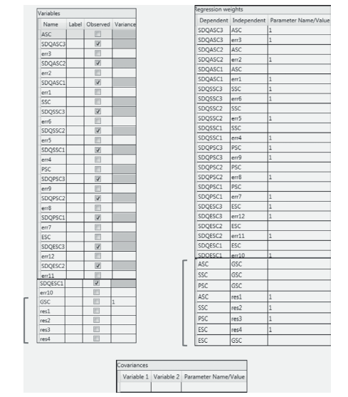
Figure 2.30 Specification of the second-order model shown in Figure 2.22 as for-matted in the Tables View optional panel.

Finally, as shown in Figure 2.30, there are no covariance specifica­tions. As noted earlier, this lack of specification results from the fact that in the specification of a second-order model, all covariation among the lower-order factors is accounted for by the higher-order factor, which is GSC in this instance.

Before moving on to our next model comprising Example 3, I wish to alert you to a couple of odd things that can happen in the building of models using both the Amos Graphics and Amos Tables View approaches. With respect to the Graphics approach, as noted earlier, the program—by default—constrains one of any congeneric set of indicator variables to 1.00. In my experience, I have found this default constraint to be typically specified for the last factor loading of any congeneric set.

Turning to the Tables View approach and to the Variables table in par­ticular, you will note a different ordering of the factor loadings between Figure 2.18 and Figure 2.30. In the first figure, I input the variables begin­ning with the first variable comprising the congeneric set of three. However, in Figure 2.30, I allowed the program to complete the table, and as you can see, it began with the third variable comprising this congeneric set. I bring this to your attention as you may have queried the possibility of errors in the tables. However, this is not the case, and the analyses will proceed in the same manner, regardless of the order in which they are listed. For a similar situation, take a look now at the Regression weights table where you will observe the rather odd specification of the higher-order loading of ESC on GSC. In lieu of being included with the other three higher-order factor loadings, it appears by itself in the last row of the table.

Based solely on my own experience with these tables, I close out this work on Example 2 with the following caveat. I think it is best to avoid trying to re-order the specified values in either the Variables or Regression weights tables once they have been entered, as otherwise, you are likely to encounter a series of error messages advising that a value already exists for the parameter you are attempting to change. Alternatively, one corrective tactic that has been found to be effective is to just delete the problematic parameter or its related fixed value and simply add it again. You should then see that it has been added to the bottom of the list. Accordingly, Amos should forget the original position and remember the new position (J. Arbuckle, personal communication, February 5, 2014).

10. Model Specification Using Amos Graphics (Example 3)

For our last example, we’ll examine a full SEM model. Recall from Chapter 1 that, in contrast to a first-order CFA model, which comprises only a measurement component, and a second-order CFA model for which the higher-order level is represented by a reduced form of a structural model, the full structural equation model encompasses both a measure­ment and a structural model. Accordingly, the full model embodies a sys­tem of variables whereby latent factors are regressed on other factors as dictated by theory and/or empirical research, as well as on the appropri­ate observed measures. In other words, in the full SEM model, certain latent variables are connected by one-way arrows, the directionality of which reflects hypotheses bearing on the causal structure of variables in the model. We turn now to the hypothesized model.

The Hypothesized Model

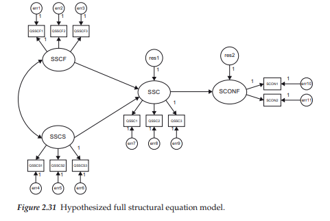
For a clearer conceptualization of full SEM models, let’s examine the rela­tively simple structure presented in Figure 2.31. The structural compo­nent of this model represents the hypothesis that a child’s self-confidence (SCONF) derives from his or her self-perception of overall social compe­tence (SSC; social SC) which, in turn, is influenced by the child’s percep­tion of how well he or she gets along with family members (SSCF), as well as with his or her peers at school (SSCS). The measurement component of the model shows each of the SC factors to have three indicator measures, and the self-confidence factor to have two.

Turning first to the structural part of the model, we can see that there are four factors. The two independent factors (SSCF; SSCS) are postulated as being correlated with each other, as indicated by the curved two-way arrow joining them, but they are linked to the other two factors by a series of regression paths, as indicated by the unidirectional arrows. Because the factors SSC and SCONF have one-way arrows pointing at them, they are easily identified as dependent variables in the model. Residual errors associated with the regression of SSC on both SSCF and SSCS, and the regression of SCONF on SSC, are captured by the disturbance terms res1 and res2, respectively. Finally, because one path from each of the two inde­pendent factors (SSCF; SSCS) to their respective indicator variables is fixed to 1.0, their variances can be freely estimated; variances of the dependent variables (SSC; SCONF), however, are not parameters in the model.

By now, you likely feel fairly comfortable in interpreting the measure­ment portion of the model, and so, substantial elaboration is not necessary here. As usual, associated with each observed measure is an error term, the variance of which is of interest. (Because the observed measures tech­nically operate as dependent variables in the model, as indicated by the arrows pointing toward them, their variances are not estimated.) Finally, to establish the scale for each unmeasured factor in the model (and for purposes of statistical identification), one parameter in each set of regres­sion paths is fixed to 1.0; recall, however, that path selection for the impos­ition of this constraint was purely arbitrary.

For this, our last example, let’s again determine if we have an iden­tified model. Given that we have 11 observed measures, we know that we have 66 (11[11 + 1]/2) pieces of information from which to derive the parameters of the model. Counting up the unknown parameters in the model, we see that we have 26 parameters to be estimated: 7 measurement regression paths; 3 structural regression paths; 2 factor variances; 11 error variances; 2 residual error variances; and 1 covariance. We therefore have 40 (66-26) degrees of freedom and, thus, an overidentified model.

Drawing the Path Diagram

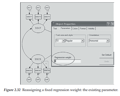
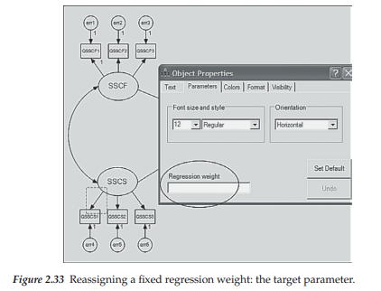
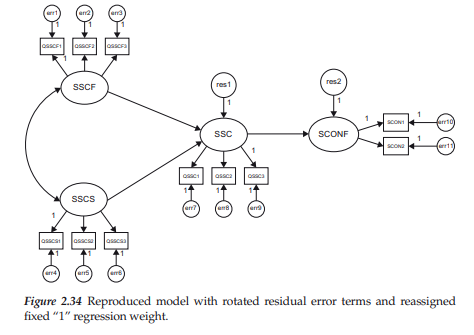
Given what you now already know about drawing path diagrams within the framework of Amos Graphics, you likely would encounter no difficulty in reproducing the hypothesized model shown in Figure 2.31. Therefore, rather than walk you through the entire drawing process related to this model, I’ll take the opportunity here to demonstrate two additional features of the drawing tools that have either not yet been illustrated or illustrated only briefly. The first of these makes use of the Object Properties icon is] in reorienting the assignment of fixed “1” values that the program automati­cally assigns to the factor loading regression paths. Turning to Figure 2.31, focus on the SSCS factor in lower left corner of the diagram. Note that the fixed path for this factor has been assigned to the one associated with the prediction of QSSCS3. For purposes of illustration, let’s reassign the fixed value of “1” to the first regression path (QSSCS1). To carry out this reori­entation process, we can either right-click on the mouse, or click on the Object Properties icon, which in either case activates the related dialog box; we focus here on the latter. In using this approach, we click first on the icon and then on the parameter of interest (QSSCS3 in this instance) which then results in the parameter value becoming enclosed in a broken line box (see Figure 2.32). Once in the dialog box, we click on the Parameter tab at the top, which then generates the dialog box shown in Figure 2.32. Note that the regression weight is listed as “1”. To remove this weight, we simply delete the value. To reassign this weight, we subsequently click on the first regression path (QSSCS1) and then on the Object Properties icon. This time, of course, the Object Properties dialog box indicates no regression weight (see Figure 2.33) and all we need to do is to add a value of “1” as shown in Figure 2.32 for indicator variable QSSCS3. Implementation of these last two actions yields a modified version of the originally hypothesized model (Figure 2.31), which is schematically portrayed in Figure 2.34.

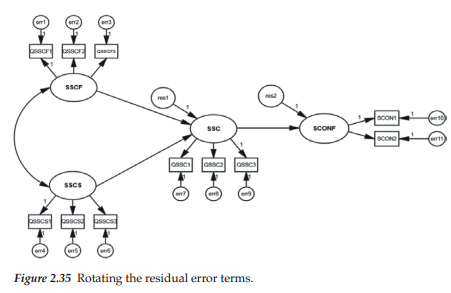
The second feature I wish to demonstrate involves the reorienta­tion of error terms, usually for purposes of improving the appearance of the path diagram. Although I briefly mentioned this procedure and showed the resulting reorientation with respect to Example 2, I consider it important to expand on my earlier illustration as it is a technique that comes in handy when you are working with path diagrams that may have many variables in the model. With the residual error terms in the 12 o’clock position, as in Figures 2.31 and 2.34, we’ll continue to click with the left mouse button until they reach the 10 o’clock position shown in Figure 2.35. Each click of the mouse results in a 45-degree clockwise move of the residual error term, with eight clicks thus returning us to the 12 o’clock position; the position indicated in Figure 2.35 resulted from seven clicks of the mouse.

Changing the Amos Default Color for Constructed Models

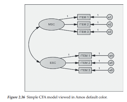
For some reason, which continues to remain a mystery to me, when you first create a figure in Amos Graphics, by program default, all components of the model are produced in a mauve/blue color. Of course, these colored models cannot be used for publication purposes. Thus, I need to show you how you can quite easily convert this default color to white (or any similar light color) of your preference.

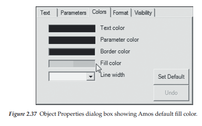
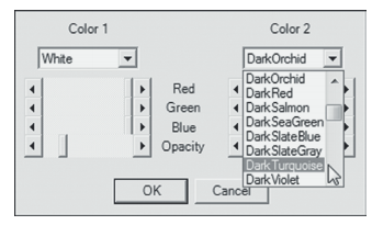
Shown in Figure 2.36 is a simple model created in Amos Graphics and shown in the original defaulted color produced by the program. To begin the change of color, click on one ellipse or rectangle in the model and then right click to bring up the Object Properties dialog box. In my case here, I clicked on the MSC ellipse. Next, click on the Color tab and move the cursor down to the Fill color rectangle as shown in Figure 2.37. Clicking on Fill color opens to a dialog box showing two sets of color panels, which are shown in Figure 2.38. On the left, you can see where I have changed the color to white. You will also need to change the color in the second panel to white. As indicated in the second panel, you will need to keep scrolling down until you reach the color “White.”

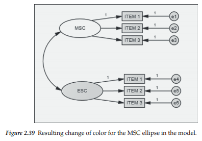
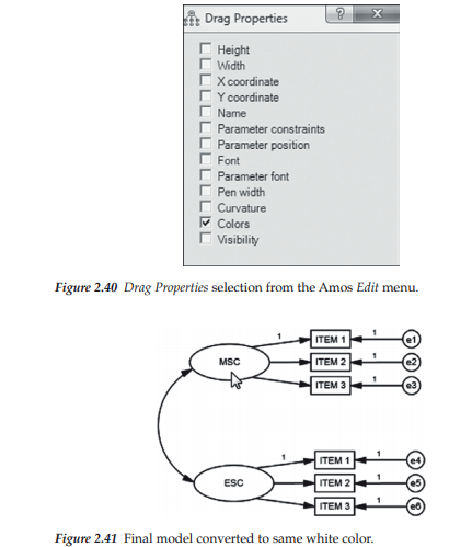
Shown in Figure 2.39, you can see that the MSC ellipse is now white. Continuing on, the next step is to click on the Edit menu and then on Select All. You will see at this point, that every symbol in the figure is high­lighted, indicating that all components have been selected. Click again on the Edit menu and then on Drag Properties, where you then put a check­mark next to the Colors square as shown in Figure 2.40. Ensure that only the Color square is checked. Next, drag the mouse pointer from the object for which you have changed the color (in this instance, the MSC ellipse) to any other ellipse or rectangle in the model. This action will result in the color of all remaining ellipses and rectangles becoming white as shown in Figure 2.41. Finally, click on Edit and then on Deselect All.

11. Model Specification Using Amos Tables View (Example 3)

Turning to the equivalent Tables View specification (see Figure 2.42) for this third example model (see Figure 2.31), you likely will have no dif­ficulty in deciphering its hypothesized parameterization as most of the specifications resemble those explained for the two previous example models. However, let’s take a look at the Regression weights table. The com­pleted cells for all variables down to, and including SCON2, should be recognizable as representing the fixed-1 values for one indicator variable
in each congeneric set, as well as for each of the error variance terms; these 1s, of course, represent their related regression paths; that is, the factor loading linking QSSCF1 to its related factor (SSCF) and the path leading from errl to the indicator variable QSSCF1.

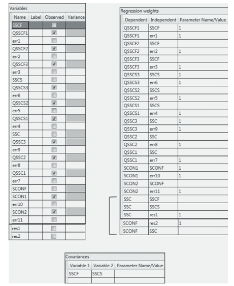
Figure 2.42 Specification of the full structural equation model shown in Figure 2.31 as formatted in the Tables View optional panel.

For clarification, I have marked only the last five rows of the Regression weights table for further explanation. The first three of these rows relate to relations among SSCF, SSCS, SSC. As can be seen, SSC is regressed on the two constructs of SSCF and SSCS, both of which serve as predictors of SSC, but with some degree of error, which is captured by the error term (resl). The regression path associated with the error term resl, therefore calls for the specification of fixed value of 1. Likewise, the same explana­tion holds for specification of a fixed 1 for residual linked to SCONF (res2).

Finally, in the Covariance table, you will see the only factor covariance in this model, which is between SSCF and SSCS.

In Chapter 1, I introduced you to the basic concepts underlying SEM and, in the present chapter, extended this information to include brief explanations of the corollary bearing on specification of a single indicator variable, as well as the issue of model identification. In this chapter, specif­ically, I have endeavored to show you the Amos Graphics approach in spe­cifying particular models under study, along with its related and newly incorporated Tables View approach. I hope that I have succeeded in giv­ing you a fairly good idea of the ease by which Amos makes this process possible. Nonetheless, it is important for me to emphasize that, although I have introduced you to a wide variety of the program’s many features, I certainly have not exhausted the total range of possibilities, as to do so would far exceed the intended scope of the present book. Now that you are fairly well equipped with knowledge of the conceptual underpinning of SEM and the basic functioning of the Amos program, let’s move on to the remaining chapters where we explore the analytic processes involved in SEM using Amos Graphics. As noted earlier, for each of the chapters to follow, I will also include the equivalent Tables View specification for­mat for each hypothesized and final model analyzed using Amos Graphics. We turn now to Chapter 3, which features an application bearing on a CFA model.

Source: Byrne Barbara M. (2016), Structural Equation Modeling with Amos: Basic Concepts, Applications, and Programming, Routledge; 3rd edition.