Application 2: Testing the Factorial Validity of Scores from a Measurement Scale (First-Order CFA Model) with AMOS

1. Key Concepts

• Assumption of multivariate normality
• The issue of multivariate outliers
• The issue of multivariate kurtosis
• Statistical strategies in addressing nonnormality
• SEM robust statistics
• Post hoc model testing and related issues
• Nested models and the chi-square difference test
• Error covariances and related issues

2. Modeling with Amos Graphics

For our second application, we once again examine a first-order confirma­tory factor analysis (CFA) model. However, this time we test hypotheses bearing on a single measuring instrument, the Maslach Burnout Inventory (MBI; Maslach & Jackson, 1981, 1986), designed to measure three dimen­sions of burnout, which the authors label Emotional Exhaustion (EE), Depersonalization (DP), and Reduced Personal Accomplishment (PA). The term “burnout” denotes the inability to function effectively in one’s job as a consequence of prolonged and extensive job-related stress; “emo­tional exhaustion” represents feelings of fatigue that develop as one’s energies become drained, “depersonalization” – the development of negative and uncaring attitudes toward others, and “reduced personal accomplishment” – a deterioration of self-confidence, and dissatisfaction in one’s achievements.

Purposes of the original study (Byrne, 1994a), from which this example is taken, were to test for the validity and invariance of factorial structure within and across gender for elementary and secondary teachers. More specifically, the intent of the study was threefold: (a) to test for the factorial validity of the MBI separately for male/female elementary and second­ary teachers, (b) to cross-validate findings across a second independent sample for each of these populations, and (c) to test for invariant factorial measurement and structure across gender for each of the two teaching panels. For the purposes of this chapter, however, only analyses bearing on the factorial validity of the MBI for a calibration sample of elementary male teachers (n = 372) are of interest.

Confirmatory factor analysis of a measuring instrument is most appropriately applied to measures that have been fully developed and their factor structures validated. The legitimacy of CFA use, of course, is tied to its conceptual rationale as a hypothesis-testing approach to data analysis. That is to say, based on theory, empirical research, or a com­bination of both, the researcher postulates a model and then tests for its validity given the sample data. Thus, application of CFA procedures to assessment instruments that are still in the initial stages of development represents a serious misuse of this analytic strategy. In testing for the validity of factorial structure for an assessment measure, the researcher seeks to determine the extent to which items designed to measure a par­ticular factor (i.e., latent construct) actually do so. In general, subscales of a measuring instrument are considered to represent the factors; all items comprising a particular subscale are therefore expected to load onto their related factor.

Given that the MBI has been commercially marketed since 1981, is the most widely used measure of occupational burnout, and has undergone substantial testing of its psychometric properties over the years (see e.g., Byrne 1991, 1993, 1994b), it most certainly qualifies as a candidate for CFA research. Interestingly, until my 1991 study of the MBI, virtually all previ­ous factor analytic work had been based only on exploratory procedures. We turn now to a description of this assessment instrument.

The Measuring Instrument under Study

The MBI is a 22-item instrument structured on a 7-point Likert-type scale that ranges from 0, “feeling has never been experienced,” to 6, “feel­ing experienced daily.” It is composed of three subscales, each meas­uring one facet of burnout; the EE subscale comprises nine items, the DP subscale five, and the PA subscale eight. The original version of the MBI (Maslach & Jackson, 1981) was constructed from data based on samples of workers from a wide range of human service organizations. Subsequently, however, Maslach and Jackson (1986), in collaboration with Schwab, developed the Educators’ Survey (MBI Form Ed), a ver­sion of the instrument specifically designed for use with teachers. The

MBI Form Ed parallels the original version of the MBI except for the modified wording of certain items to make them more appropriate to a teacher’s work environment.

3. The Hypothesized Model

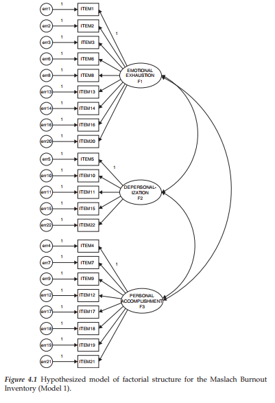
The CFA model of MBI structure hypothesizes a priori that (a) responses to the MBI can be explained by three factors—EE, DP, and PA; (b) each item has a nonzero loading on the burnout factor it was designed to measure, and zero loadings on all other factors; (c) the three factors are correlated; and (d) the error/uniqueness terms associated with the item measurements are uncorrelated. A schematic representation of this model is shown in Figure 4.I.¹

This hypothesized 3-factor model of MBI structure provides the Amos Graphics specifications for the model to be tested here. In Chapter 2, we reviewed the process involved in computing the number of degrees of free­dom and, ultimately, in determining the identification status of a hypothe­sized model. Although all such information (estimated/fixed parameters; degrees of freedom) is provided in the Model/Parameter Summary dialog boxes of the Amos output, I strongly encourage you to make this practice part of your routine, as I firmly believe that it not only forces you to think through the specification of your model, but also may serve you well in resolving future problems that may occur down the road. In the present case, the sample covariance matrix comprises a total of 253 (23 x 22/2) pieces of information (or sample moments). Of the 72 parameters in the model, only 47 are to be freely estimated (19 factor loadings, 22 error vari­ances, 3 factor variances, and 3 factor covariances); all others (25) are fixed parameters in the model (i.e., they are constrained to equal zero or some nonzero value). As a consequence, the hypothesized model is overidenti­fied with 206 (253 – 47) degrees of freedom.

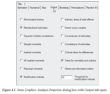
Prior to submitting the model input to analysis, you will likely wish to review the Analysis Properties box (introduced in Chapter 3) in order to tailor the type of information to be provided in the Amos output on esti­mation procedures, and/or on many other aspects of the analysis. At this time, we are only interested in output file information. Recall that clicking on the Analysis Properties icon [HD] and then on the “Open” tab yields the dialog box shown in Figure 4.2. For our purposes here, we request the modifications indices (MIs), the standardized parameter estimates (pro­vided in addition to the unstandardized estimates, which are default), and tests for normality and outliers, all of which are options you can choose when the Output tab is activated. Consistent with the MI specification in Chapter 3, we’ll again stipulate a threshold of 10. Thus, only MI estimates equal to or greater than 10 will be included in the output file.

Having specified the hypothesized 3-factor CFA model of MBI struc­ture, located the data file to be used for this analysis (as illustrated in Chapter 3), and selected the information to be included in the reporting of results, we are now ready to analyze the model

Selected Amos Output: The Hypothesized Model

In contrast to Chapter 3, which served the purpose of a fully documented introduction to the Amos output file, only selected portions of this file will be reviewed and discussed here as well as for all remaining chapters. We examine first, the model summary, assessment of normality and case outliers, indices of fit for the model as a whole, and finally, modification indices (MIs) as a means of pinpointing areas of model misspecification.

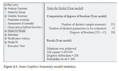
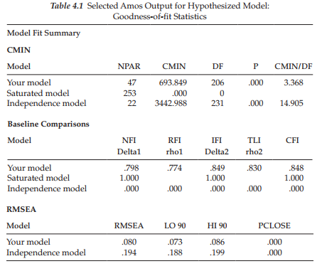
Model summary. In reviewing the analytic summary shown in Figure 4.3, we see that estimation of the hypothesized model resulted in an overall x² value of 693.849 with 206 degrees of freedom and a probabil­ity value of .000. Of import also is the notation that the Minimum was achieved. This latter statement indicates that Amos was successful in esti­mating all model parameters thereby resulting in a convergent solution.

If, on the other hand, the program had not been able to achieve this goal, it would mean that it was unsuccessful in being able to reach the minimum discrepancy value, as defined by the program in its comparison of the sample covariance and restricted covariance matrices. Typically, an out­come of this sort results from incorrectly specified models and/or data in which there are linear dependencies among certain variables.

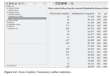
Assessment of multivariate outliers. Outliers represent cases for which scores are substantially deviant from all the others in a particular set of data. A univariate outlier has an extreme score on a single variable whereas a multivariate outlier has extreme scores on two or more variables (Kline, 2011). A common approach to the detection of multivariate outliers is the computation of the squared Mahalanobis distance (d²) for each case. This statistic measures the distance in standard deviation units between a set of scores for one case and the sample means for all variables (centroids). Typically, an outlying case will have a d² value that stands distinctively apart from all other d² values. Looking back at Figure 4.3, you will see “Observations farthest from the centroid…” entered on the line below “Assessment of normality.” Clicking on this line provides you with the information needed for determining the presence of multivariate outliers. From a review of these values reported in Figure 4.4, we can conclude that there is minimal evidence of serious multivariate outliers in these data.

Assessment of nonnormality. A critically important assumption in the conduct of SEM analyses in general, and in the use of Amos in particular (Arbuckle, 2015), is that the data are multivariate normal. This requirement is rooted in large sample theory from which the SEM methodology was spawned. Thus, before any analyses of data are undertaken, it is important to check that this criterion has been met. Particularly problematic to SEM analyses are data that are multivariate kurtotic, the situation where the multivariate distribution of the observed variables has both tails and peaks that differ from those characteristic of a multivariate normal distribution (see Raykov & Marcoulides, 2000). More specifically, in the case of multi­variate positive kurtosis, the distributions will exhibit peakedness together with heavy (or thick) tails; conversely, multivariate negative kurtosis will yield flat distributions with light tails (De Carlo, 1997). To exemplify the most commonly found condition of multivariate kurtosis in SEM, let’s take the case of a Likert-scaled questionnaire, for which responses to certain items result in the majority of respondents selecting the same scale point. For each of these items, the score distribution would be extremely peaked (i.e., leptokurtic); considered jointly, these particular items would reflect a multivariately positive kurtotic distribution. (For an elaboration of both univariate and multivariate kurtosis, readers are referred to DeCarlo, 1997.)

Prerequisite to the assessment of multivariate normality is the need to check for univariate normality as the latter is a necessary, although not suf­ficient, condition for multivariate normality (DeCarlo, 1997). Thus, we turn now to the results of our request on the Analysis Properties dialog box (see Figure 4.2) for an assessment of normality as it relates to the male teacher data used in this application. These results are presented in Figure 4.5.

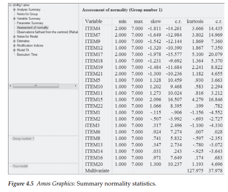
Statistical research has shown that whereas skewness tends to impact tests of means, kurtosis severely affects tests of variances and covariances (DeCarlo, 1997). Given that SEM is based on the analysis of covariance structures, evidence of kurtosis is always of concern and in particular, evi­dence of multivariate kurtosis, as it is known to be exceptionally detrimen­tal in SEM analyses. With this in mind and turning first to the univariate statistics, we focus only on the last two columns of Figure 4.5, where we find the univariate kurtosis value and its critical ratio (i.e., Z-value) listed for each of the 22 MBI items. As shown, positive values range from .007 to 5.100 and negative values from -.597 to -1.156, yielding an overall mean univariate kurtosis value of 1.091. The standardized kurtosis index (p₂) in a normal distribution has a value of 3, with larger values representing posi­tive kurtosis and lesser values representing negative kurtosis. However, computer programs typically rescale this value by subtracting 3 from the p₂ value thereby making zero the indicator of normal distribution and its sign the indicator of positive or negative kurtosis (DeCarlo, 1997; Kline, 2011; West, Finch, & Curran, 1995). Although there appears to be no clear consensus as to how large the nonzero values should be before conclusions
of extreme kurtosis can be drawn (Kline, 2011), West et al. (1995) consider rescaled p₂ values equal to or greater than 7 to be indicative of early depar­ture from normality. Using this value of 7 as guide, a review of the kurtosis values reported in Figure 4.5 reveals no item to be substantially kurtotic.

Of import is the fact that although the presence of nonnormal observed variables precludes the possibility of a multivariate normal distribution, the converse is not necessarily true. That is, regardless of whether the dis­tribution of observed variables is univariate normal, the multivariate dis­tribution can still be multivariate nonnormal (West et al., 1995). Thus, we turn now to the index of multivariate kurtosis and its critical ratio, which appear at the bottom of the kurtosis and critical ratio (C.R.) columns, respectively. Of most import here is the C.R. value, which in essence repre­sents Mardia’s (1970, 1974) normalized estimate of multivariate kurtosis, although it is not explicitly labeled as such (J. Arbuckle, personal commu­nication, March 2014). When the sample size is very large and multivari­ately normal, Mardia’s normalized estimate is distributed as a unit normal variate such that large values reflect significant positive kurtosis and large negative values reflect significant negative kurtosis. Bentler (2005) has suggested that, in practice, normalized estimates >5.00 are indicative of data that are nonnormally distributed. In this application, the z-statistic of 37.978 is highly suggestive of multivariate nonnormality in the sample.

Addressing the presence of nonnormal data. When continuous (ver­sus categorical) data reveal evidence of multivariate kurtosis, inter­pretations based on the usual ML estimation may be problematic and thus an alternative method of estimation is likely more appropriate. One approach to the analysis of nonnormal data is to base analyses on asymptotic distribution-free (ADF) estimation (Browne 1984a), which is available in Amos by selecting this estimator from those offered on the Estimation tab of the Analysis Properties icon or drop-down View menu. However, it is now well known that unless sample sizes are extremely large (1,000 to 5,000 cases; West et al., 1995), the ADF estimator performs very poorly and can yield severely distorted estimated values and stand­ard errors (Curran et al., 1996; Hu, Bentler, & Kano, 1992; West et al., 1995). More recently, statistical research has suggested that, at the very least, sample sizes should be greater than 10 times the number of esti­mated parameters, otherwise the results from the ADF method generally cannot be trusted (Raykov & Marcoulides, 2000). (See Byrne, 1995 for an example of the extent to which estimates can become distorted using the ADF method with a less than adequate sample size.) As shown in Figure 4.4, the model under study in this chapter has 47 freely estimated parameters, suggesting a minimal sample size of 470. Given that our current sample size is 372, we cannot realistically use the ADF method of estimation.

In contrast to the ADF method of estimation, Chou, Bentler, and Satorra (1991) and Hu et al. (1992) have argued that in analyses of nonnormal data it may be more appropriate to correct the test statistic, rather than use a differ­ent mode of estimation. Based on maximum likelihood estimation, which is typically default in SEM software programs, Satorra and Bentler (1988, 1994) developed such a statistic that incorporates a scaling correction for both the x² statistic and the estimated parameter standard errors when dis­tributional assumptions are violated. Computation of this corrected x² (com­monly termed the Satorra-Bentler chi-square [S-B x²]) takes into account the model, the estimation method, and the sample kurtosis values, and has been shown to be the most reliable test statistic for evaluating mean and covariance structure models under various distributions and sample sizes (Hu et al., 1992; Curran et al., 1996). Given that the Satorra-Bentler correc­tion procedure enables statistically sound tests of hypothesized models in the face of nonnormally distributed data, it is regarded as a robust approach to the analyses of SEM models; relatedly, the S-B x² is categorized as, and commonly referred to as, a robust statistic and the corrected standard error estimates are termed “robust” estimates. Although such correction of the ML estimator is considered to be the most straightforward strategy when the assumption of multivariate normality is violated (Finney & DiStefano, 2006), unfortunately this option is not available in the Amos program.

Kline (2011) suggests that yet another option in the testing of models based on nonnormal data is the use of bootstrapping, a statistical procedure that falls under the broader rubric of resampling. Within this framework, the models are tested using normal theory ML estimation, albeit with nonparametric (i.e., distribution-free; no assumption of normality) boot­strapping. As such, the only assumption is that the population and sample distributions have the same shape. Several readers have enquired about use of the Bollen-Stine (Bollen & Stine, 1992, 1993) bootstrapping proced­ure in Amos as an aid to addressing the issue of nonnormality. However, it is important to realize that this procedure is not designed to test for nor­mality (J. Arbuckle, personal communication, March 2014). Rather, it tests for the correctness of a hypothesized model without assuming normality. Furthermore, the Bollen-Stine procedure does not make any correction to the standard errors given data that are nonnormally distributed.

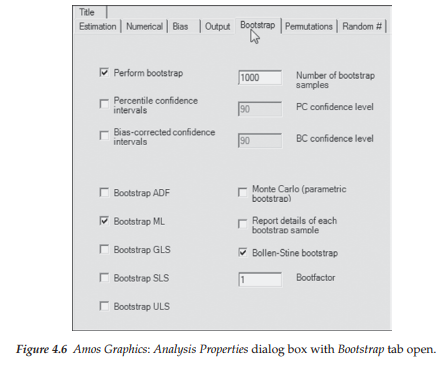
For a brief look at the Amos output resulting from implementation of the Bollen-Stine procedure, let’s once again test the hypothesized model of the MBI (see Figure 4.1) using the same specifications as per the Output tab shown in Figure 4.2. In addition, however, we now request the Bollen-Stine bootstrap procedure by first clicking on the Bootstrap tab and then selecting the specific information shown in Figure 4.6. As shown here, I have requested the program to perform this Bollen-Stine bootstrap analysis based on 1,000 samples. The results of this bootstrapping action are shown in Figure 4.7.

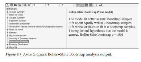
Let’s now interpret these results. The information provided tells us that the program generated 1,000 datasets from an artificial population in which the specified model is correct and the distribution of measured var­iables is consistent with that of the original sample. We are advised that the model fit better in 1,000 bootstrap samples than it did in the original sample. Said another way, all 1,000 randomly generated datasets fitted the model better that the actual real dataset. That is, if you ranked 1,001 datasets (the original dataset plus the 1,000 generated data sets), the real dataset would be the worst of the 1,001 sets. In terms of probability, the results imply that the likelihood of this happening by chance if the spe­cified model holds in the real population is 1/1,000 (.0010). Thus, we can reject the null hypothesis that the specified model is correct (in the real population) with probability = .001.

From a review of these bootstrapping results, it is clear that the only information reported bears on the extent to which the model fits the data. Thus, I consider further discussion of the so-called bootstrapping option to yield no particular benefits in testing for the factorial validity of the MBI based on data that are somewhat nonnormally distributed. However, for readers who may be interested in learning further how bootstrapping might be applied in dealing with nonnormal data, I provide a more exten­sive overview and application of bootstrapping in general, and of the Bollen-Stine bootstrapping procedure in particular, in Chapter 12.

Provided with no means of correcting the standard error estimates in Amos, we will continue to base our analyses on ML estimation. However, given that I have analyzed the same data using the Satorra-Bentler robust approach in both the EQS and Mplus programs (Byrne, 2006, 2012, respectively)² I believe that it may be both instructive and helpful for you to view the extent to which results deviate between the normal-theory ML and corrected ML estimation methods. Thus an extended discussion of the Satorra-Bentler robust approach, together with a brief comparison of both the overall goodness-of-fit and selected parameter statistics related to the final model, is presented at the end of this chapter.

Model Evaluation

Goodness-of-fit summary. Because the various indices of model fit provided by the Amos program were discussed in Chapter 3, model evaluation throughout the remaining chapters will be limited to those summarized in Table 4.1. These criteria were chosen on the basis of (a) their variant approaches to the assessment of model fit (see Hoyle, 1995b), and (b) their support in the literature as important indices of fit that should be reported.³ This selection, of course, in no way implies that the remaining criteria are unimportant. Rather, it addresses the need for users to select a subset of goodness-of-fit indices from the generous quantity provided by the Amos program.⁴ These selected indices of fit are presented in Table 4.1.

In reviewing these criteria in terms of their optimal values (see Chapter 3), we can see that they are consistent in their reflection of an ill-fitting model. For example, the CFI value of .848 is indicative of an extremely poor fit of the model to the data. Thus, it is apparent that some modification in specification is needed in order to identify a model that better represents the sample data. To assist us in pinpointing possible areas of misfit, we examine the modification indices. Of course, as noted in Chapter 3, it is important to realize that once we have determined that the hypothesized model represents a poor fit to the data (i.e., the null hypothesis has been rejected), and then proceed in post hoc model fitting to identify areas of misfit in the model, we cease to operate in a confirma­tory mode of analysis. All model specification and estimation henceforth represent exploratory analyses.

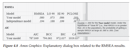
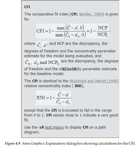
Before we examine the MIs as markers of possible model misspeci- fication, however, let’s divert briefly to review the explanatory dialog box pertinent to the PCLOSE statistic associated with the RMSEA, which was generated by clicking on the .000 for “Your model,” and is shown in Figure 4.8. It is important to note, however, that this dialog box repre­sents only one example of possible explanations made available by the program. In fact, by clicking on any value or model-fit statistic reported in the Model Fit section of the Amos output (of which Table 4.1 shows only a small portion, but see Chapter 3 for a complete listing of possible output information), you can access its related explanatory dialog box. As one example, clicking on the CFI index of fit yields the full statistical explan­ation of this index shown in Figure 4.9.

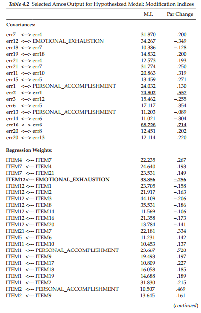
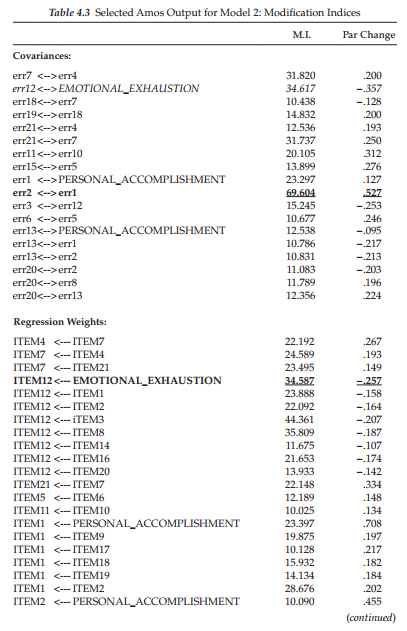
Modification indices. We turn now to the MIs presented in Table 4.2. Based on the initially hypothesized model (Model 1), all factor loadings and error covariance terms that were fixed to a value of 0.0 are of substan­tial interest as they represent the only meaningful sources of misspecifica- tion in a CFA model. As such, large MIs argue for the presence of factor cross-loadings (i.e., a loading on more than one factor)⁵ and error covari­ances, respectively. Consistently with other SEM programs, Amos com­putes an MI for all parameters implicitly assumed to be zero, as well as for those that are explicitly fixed to zero or some other nonzero value. In reviewing the list of MIs in Table 4.2, for example, you will see suggested regression paths between two observed variables (e.g., ITEM4 ^ ITEM7) and suggested covariances between error terms and factors (e.g., err12 ^ EMOTIONAL EXHAUSTION), neither of which makes any substantive sense. Given the meaninglessness of these MIs, then, we focus solely on those representing cross-loadings and error covariances.

Turning first to the MIs related to the Covariances (in contrast to other SEM programs, these precede the Regression weights in the Amos output), we see very clear evidence of misspecification associated with the pairing of error terms associated with Items 1 and 2 (err2 ^ errl; MI = 74.802) and those associated with Items 6 and 16 (err16 ^ err6; MI = 88.728). Although, admittedly, there are a few additionally quite large MI values shown, these two stand apart in that they are substantially larger than the others; they represent misspecified error covariances⁶. These measurement error covariances represent systematic, rather than random measurement error in item responses and they may derive from characteristics specific either to the items, or to the respondents (Aish & Joreskog, 1990). For example, if these parameters reflect item characteristics, they may represent a small omitted factor. If, on the other hand, they represent respondent character­istics, they may reflect bias such as yea/nay-saying, social desirability, and the like (Aish & Joreskog, 1990). Another type of method effect that can trigger error covariances is a high degree of overlap in item content. Such redundancy occurs when an item, although worded differently, essen­tially asks the same question. I believe the latter situation to be the case here. For example, Item 16 asks whether working with people directly, puts too much stress on the respondent, while Item 6 asks whether work­ing with people all day puts a real strain on him/her.

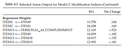
Although a review of the MIs for the Regression weights (i.e., fac­tor loadings) reveals four parameters indicative of cross-loadings (ITEM12 ← EMOTIONAL EXHAUSTION; ITEM1 ← PERSONAL ACCOMPLISHMENT; ITEM2 ← PERSONAL ACCOMPLISHMENT; ITEM13 ← PERSONAL ACCOMPLISHMENT), I draw your attention to the one with the highest value (MI = 33.856), which is highlighted in bold­face type.⁸ This parameter, which represents the cross-loading of Item 12 on the EE factor, stands apart from the three other possible cross-loading misspecifications. Such misspecification, for example, could mean that Item 12, in addition to measuring personal accomplishment, also meas­ures emotional exhaustion; alternatively, it could indicate that, although Item 12 was postulated to load on the PA factor, it may load more appro­priately on the EE factor.

5. Post Hoc Analyses

Provided with information related both to model fit and to possible areas of model misspecification, a researcher may wish to consider respecifying an originally hypothesized model. As emphasized in Chapter 3, should this be the case, it is critically important to be cognizant of both the exploratory nature of, and the dangers associated with the process of post hoc model fitting. Having determined (a) inadequate fit of the hypothesized model to the sample data, and (b) at least two misspecified parameters in the model (i.e., the two error covariances previously specified as zero), it seems both reasonable and logical that we now move into exploratory mode and attempt to modify this model in a sound and responsible manner. Thus, for didactic purposes in illustrating the various aspects of post hoc model fitting, we’ll proceed to respecify the initially hypothesized model of MBI structure taking this information into account.

Model respecification that includes correlated errors, as with other parameters, must be supported by a strong substantive and/or empirical rationale (Joreskog, 1993) and I believe that this condition exists here. In light of (a) apparent item content overlap, (b) the replication of these same error covariances in previous MBI research (e.g., Byrne, 1991, 1993), and (c) Bentler and Chou’s (1987) admonition that forcing large error terms to be uncorrelated is rarely appropriate with real data, I consider respecifica­tion of this initial model to be justified. Testing of this respecified model (Model 2) now falls within the framework of post hoc analyses.

Let’s return now to Amos Graphics and the respecification of Model 1 in structuring Model 2.

6. Model 2

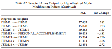
Respecification of the hypothesized model of MBI structure involves the addition of freely estimated parameters to the model. However, because the estimation of MIs in Amos is based on a univariate approach (as are the LISREL and Mplus programs, but in contrast to the EQS program, which takes a multivariate approach), it is critical that we add only one parameter at a time to the model as the MI values can change substantially from one tested parameterization to another. Thus, in building Model 2, it seems most reasonable to proceed first in adding to the model the error covariance having the largest MI. As shown in Table 4.2, this param­eter represents the error terms for Items 6 and 16 and, according to the Parameter Change statistic, should result in a parameter estimated value of approximately .714. Of related interest is the section in Table 4.2 labeled Regression weights, where you see highlighted in bold italic type two sug­gested regression paths. Although technically meaningless, because it makes no substantive sense to specify these two parameters (ITEM6 ^ ITEM16; ITEM16 ^ ITEM6), I draw your attention to them only as they reflect on the problematic link between Items 6 and 16. More realistically, this issue is addressed through the specification of an error covariance.

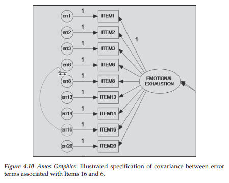
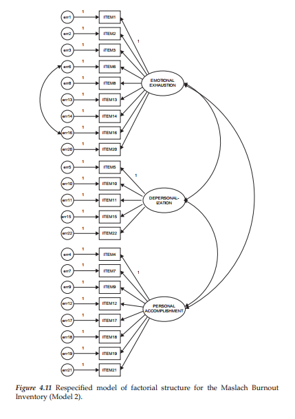
Turning to Amos Graphics, we modify the initially hypothesized model by adding a covariance between these Item 16 and Item 6 error terms by first clicking on the Draw Covariances icon [0], then on errl6, and finally, on err6 as shown in Figure 4.10. The modified model structure for Model 2 is presented in Figure 4.11.

Selected Amos Output: Model 2

Goodness-of-fit statistics related to Model 2 reveal that incorporation of the error covariance between Items 6 and 16 made a substantially large improvement to model fit. In particular, we can note decreases in the overall chi-square from 693.849 to 596.124 and the RMSEA from .080 to .072, as well as an increase in the CFI value from .848 to .878.⁹ In assess­ing the extent to which a respecified model exhibits improvement in fit, it has become customary when using a univariate approach, to determine if the difference in fit between the two models is statistically significant. As such, the researcher examines the difference in x² (Ax²) values between the two models. Doing so, however, presumes that the two models are nested.¹⁰ The differential between the models represents a measurement of the overidentifying constraints and is itself x²-distributed, with degrees of freedom equal to the difference in degrees of freedom (Adf); it can thus be tested statistically, with a significant Ax² indicating substantial improve­ment in model fit. This comparison of nested models is technically known as the Chi-square Difference Test. Comparison of Model 2 (x² (₂₀₅) = 596.124) with Model 1 (x²(₂₀₆)=693.849), for example, yields a difference in x² value (Ax²(i)) of 97.725.¹¹

The unstandardized estimate for this error covariance parameter is .733, which is highly significant (C.R. = 8.046) and even larger than the predicted value suggested by the Parameter Change statistic noted ear­lier; the standardized parameter estimate is .497 thereby reflecting a very strong error correlation!

Turning to the resulting MIs for Model 2 (see Table 4.3), we observe that the error covariance related to Items 1 and 2 remains a strongly misspecified parameter in the model, with the estimated parameter change statistic suggesting that if this parameter were incorporated into the model, it would result in an estimated value of approximately .527. As with the error covariance between Items 6 and 16, the one between Items 1 and 2 suggests redundancy due to content overlap. Item 1 asks if the respondent feels emotionally drained from his or her work whereas Item 2 asks if the respondent feels used up at the end of the workday. Clearly, there appears to be an overlap of content between these two items.

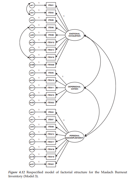
Given the strength of this MI and again, the obvious overlap of item content, I recommend that this error covariance parameter also be included in the model. This modified model (Model 3) is shown in Figure 4.12.

7. Model 3

Selected Amos Output: Model 3

Goodness-of-fit statistics related to Model 3 again reveal a statistically significant improvement in model fit between this model and Model 2 (x²(₂₀₄) = 519.082; Δχ2(1) = 77.04), and substantial differences in the CFI (.902 vs. .878) and RMSEA (.065 vs. .072) values.

Turning to the MIs, which are presented in Table 4.4, we see that there are still at least two error covariances with fairly large MIs (err7 ↔ err4 and err 21 ↔err7). However, in reviewing the items associated with these two error parameters, I believe that the substantive rationale for their inclusion is very weak and therefore they should not be considered for addition to the model. On the other hand, I do see reason for consider­ing the specification of a cross-loading with respect to Item 12 on Factor 1. In the initially hypothesized model, Item 12 was specified as loading on Factor 3 (Reduced Personal Accomplishment), yet the MI is telling us that this item should additionally load on Factor 1 (Emotional Exhaustion). In trying to understand why this cross-loading might be occurring, let’s take a look at the essence of the item content, which asks for a level of agreement or disagreement with the statement that the respondent “feels very energetic.”

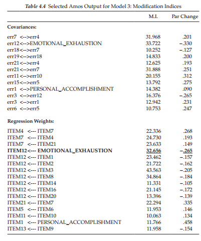
Although this item was deemed by Maslach and Jackson (1981, 1986) to measure a sense of personal accomplishment, it seems both evident and logical that it also taps one’s feelings of emotional exhaustion. Ideally, items on a measuring instrument should clearly target only one of its underly­ing constructs (or factors). The question related to our analysis of the MBI, however, is whether or not to include this parameter in a third respecified model. Provided with some justification for the double-loading effect, together with evidence from the literature that this same cross-loading has been noted in other research, I consider it appropriate to respecify the model (Model 4) with this parameter freely estimated.

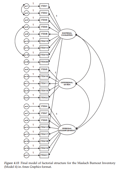
In modifying Model 3 to include the cross-loading of Item 12 on Factor 1 (Emotional Exhaustion), we simply use the Draw Paths icon [0] to link the two. The resulting Model 4 is presented in Figure 4.13.

8. Model 4

Selected Amos Output: Model 4

Not unexpectedly, goodness-of-fit indices related to Model 4 show a fur­ther statistically significant drop in the chi-square value from that of Model 3 (x²(2₀3) = 477.298; Ay²(₁) = 41.784). Likewise there is evident improvement from Model 3 with respect to both the RMSEA (.060 vs. .065) and the CFI (.915 vs. .902).

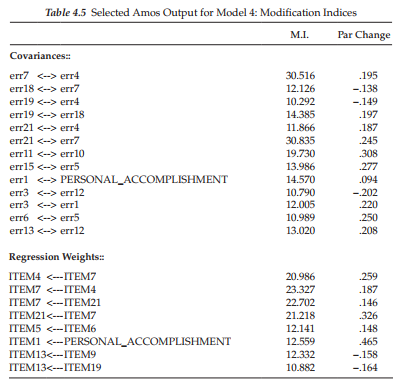
With respect to the MIs, which are shown in Table 4.5, I see no evidence of substantively reasonable misspecification in Model 4. Although, admit­tedly, the fit of .92 is not as high as I would like it to be, I am cognizant of the importance of modifying the model to include only those parameters that are substantively meaningful and relevant. Thus, on the basis of findings related to the test of validity for the MBI, I consider Model 4 to represent the final best-fitting and most parsimonious model to represent the data.

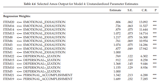
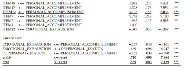
Finally, let’s examine both the unstandardized, and the standard­ized factor loadings, factor covariances, and error covariances, which are presented in Tables 4.6 and 4.7, respectively. We note first that in review­ing the unstandardized estimates, all are statistically significant given C.R. values >1.96.

Turning first to the unstandardized factor loadings, it is of particu­lar interest to examine results for Item 12 for which its targeted load­ing was on Personal Accomplishment (Factor 3) and its cross-loading on Emotional Exhaustion (Factor 1). As you will readily observe, the load­ing of this item on both factors is not only statistically significant, but in addition, is basically of the same degree of intensity. In checking its unstandardized estimate in Table 4.6, we see that the critical ratio for both parameters is almost identical (6.035 vs. -6.389), although one has a posi­tive sign and one a negative sign. Given that the item content states that the respondent feels very energetic, the negative path associated with the Emotional Exhaustion factor is perfectly reasonable. Turning to the related standardized estimates in Table 4.7, it is interesting to note that the estimated value for the targeted loading (.425) is only slightly higher than it is for the cross-loading (-.324), both being of moderate strength.

Presented with these findings and maintaining a watchful eye on parsimony, it behooves us at this point to test a model in which Item 12 is specified as loading onto the alternate factor (Emotional Exhaustion), rather than the one on which it was originally designed to load (Personal Accomplishment); as such, there is now no specified cross-loading. In the interest of space, however, I simply report the most important cri­teria determined from this alternate model (Model 3a) compared with Model 3 (see Figure 4.8) in which Item 12 was specified as loading on Factor 3, its original targeted factor. Accordingly, findings from the esti­mation of this alternative model revealed (a) the model to be slightly less well-fitting (CFI = .895) than for Model 3 (CFI = .902), and (b) the stand­ardized estimate to be weaker (-.468) than for Model 3 (.554). As might be expected, a review of the MIs identified the loading of Item 12 on Factor 3 (MI = 49.661) to be the top candidate for considered respecification in a subsequent model; by comparison, the related MI in Model 3 was 32.656  and identified the loading of Item 12 on Factor 1 as the top candidate for
respecification (see Table 4.4).

From these comparative results between Model 3 and Model 3a (the alternative model), it seems evident that Item 12 is problematic and defin­itely in need of content revision, a task that is definitely out of my hands. Thus, provided with evidence of no clear loading of this item, it seems most appropriate to leave the cross-loading in place.

Comparison with Robust Analyses Based on the Satorra-Bentler Scaled Statistic

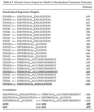
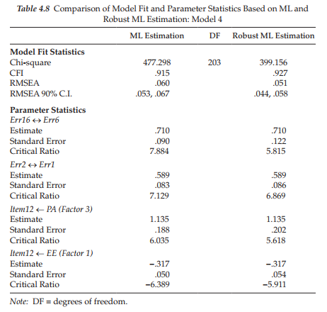
Given that the analyses in this chapter were based on the default normal theory ML estimation method with no consideration of the multivari­ate nonnormality of the data noted earlier, I consider it both interest­ing and instructive to compare the overall goodness-of-fit pertinent to Model 4, as well as key statistics related to a selected few of its esti­mated parameters. The major thrust of the S-B Robust ML approach in addressing nonnormality, as noted briefly at the beginning of this chap­ter, is that it provides a scaled statistic (S-Bx²) which corrects the usual ML x² value, as well as the standard errors (Satorra & Bentler, 1988, 1994; Bentler & Dijkstra, 1985). Although the ML estimates will remain the same for both programs, the standard errors of these estimates will differ in accordance with the extent to which the data are multivariate nonnormal. Because the critical ratio represents the estimate divided by its standard error, the corrected critical ratio for each parameter may ultimately lead to different conclusions regarding its statistical signifi­cance. This comparison of model fit, as well as parameter statistics, are presented in Table 4.8.

Turning first to the goodness-of-fit statistics, it is evident that the S-B corrected chi-square value is substantially lower than that of the uncor­rected ML value (399.156 vs. 477.298). Such a large difference between the two chi-square values provides evidence of substantial nonnormality of the data. Because calculation of the CFI necessarily involves the x² value, you will note also a substantial increase in the robust CFI value (.927 vs. .915). Finally, we note that the corrected RMSEA value is also lower (.044) than its related uncorrected value (.060).

In reviewing the parameter statistics, it is interesting to note that although the standard errors underwent correction to take nonnormal­ity into account, thereby yielding critical ratios that differed across the Amos and EQS programs, the final conclusion regarding the statistical significance of the estimated parameters remains the same. Importantly, however, it should be noted that the uncorrected ML approach tended to overestimate the degree to which the estimates were statistically sig­nificant. Based on this information, we can feel confident that, although we were unable to directly address the issue of nonnormality in the data for technical reasons, and despite the tendency of the uncorrected ML estimator to overestimate the statistical significance of these estimates, overall conclusions were consistent across CFA estimation approaches in suggesting Model 4 to most appropriately represent MBI factorial structure.

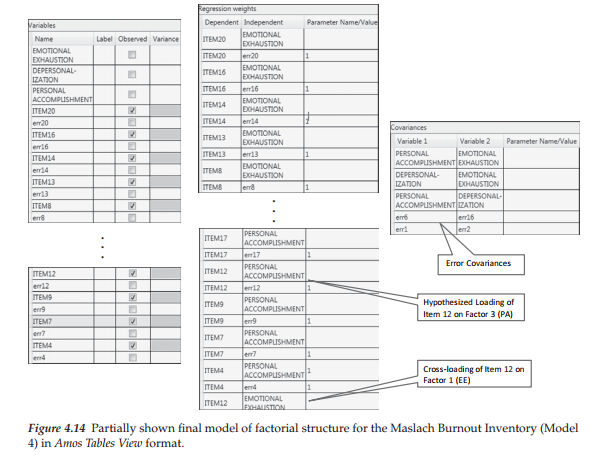
9. Modeling with Amos Tables View

Let’s turn now to Figure 4.14 in which the same final Model 4 is shown in Tables View format. Although the three tables comprising this format are included here, due to the length of the Variables and Regression weights tables, I was unable to include all parameters; the three dots indicate the location of the missing cells. The Variables table is very straightforward with all checked cells representing all items (i.e., the observed variables). Turning to the Regression weights table, you will observe that the regres­sion path for each error term has been fixed to a value of 1.0, as indicated in the “Parameter Name/Value” column, which of course is consistent with the path diagram representing all models tested. The item of interest in this table is Item 12, as it was found to load on the hypothesized fac­tor of Personal Accomplishment (F3) and to cross-load onto the factor of Emotional Exhaustion (F1). Finally, as shown in the Covariances table, in addition to the hypothesized covariance among each of the three latent factors, the error variances associated with Items 6 and 16, and with Items 1 and 2 also were also found to covary.

Source: Byrne Barbara M. (2016), Structural Equation Modeling with Amos: Basic Concepts, Applications, and Programming, Routledge; 3rd edition.