Analysis of Variance with SPSS – Problem 10.3: Nonparametric Kruskal-Wallis Test

What else can you do if the homogeneity of variance assumption is violated (or if your data are ordinal or highly skewed)? One answer is a nonparametric statistic. Let’s make comparisons similar to Problem 10.1, assuming that the data are ordinal or the assumption of equality of group variances is violated. Remember that the variances for the three fathers’ education groups were significantly different on math achievement, and the competence scale was not normally distributed (see Chapter 4). The assumptions of the Kruskal-Wallis test are the same as for the Mann-Whitney test (see Chapter 9).

• Are there statistically significant differences among the three father’s education groups on math achievement and the competence scale?

Follow these commands:

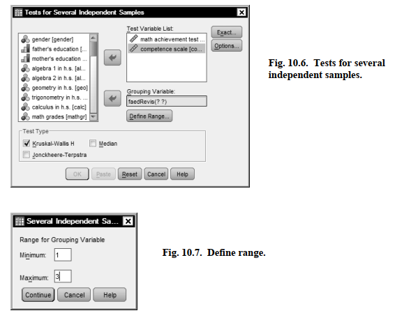
• Analyze → Nonparametric Tests → Legacy Dialogs → K Independent Samples…
• Move the dependent variables of math achievement and competence to the Test Variable List: (see Fig. 10.6).
• Move the independent variable father’s educ revised to the Grouping Variable
• Click on Define Range and insert 1 and 3 into the minimum and maximum boxes (Fig. 10.7) because faedRevis has values of 1, 2, and 3.
• Click on Continue.
• Ensure that Kruskal-Wallis H (under Test Type) in the main dialogue box is checked.
• Then click on OK. Do your results look like Output 10.3?

Output 10.3: Kruskal-Wallis Nonparametric Tests

NPAR TESTS

/K-W=mathach competence BY faedRevis(1 3)

/MISSING ANALYSIS.

NPar Tests

Interpretation of Output 10.3

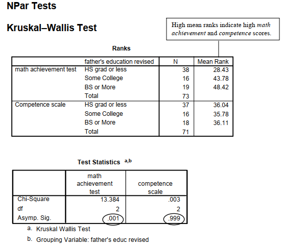
As in the case of the Mann-Whitney test (Chapter 9), the Ranks table provides Mean Ranks for the two dependent variables, math achievement and competence. In this case, the Kruskal- Wallis (K-W) test will compare the mean ranks for the three father’s education groups.

The Test Statistics table shows whether there is an overall difference among the three groups. Notice that the p (Asymp. Sig.) value for math achievement is .001, which is the same as it was in Output 10.1 using the one-way ANOVA. This is because K-W and ANOVA have similar power to detect a difference. Note also that there is not a significant difference among the father’s education groups on the competence scale (p = .999).

Unfortunately, there are no post hoc tests built into the K-W test, as there are for the one-way ANOVA. Thus, you cannot tell which of the pairs of father’s education means are different on math achievement. One method to check this would be to run three Mann-Whitney (M-W) tests comparing each pair offather’s education mean ranks (see Problem 9.3). Note you would only do the post hoc M-W tests if the K-W test was statistically significant; thus, you would not do the M-W for competence. It also would be prudent to adjust the significance level by dividing .05 by 3 (the Bonferonni correction) so that you would require that the M-W Sig. be < .017 to be statistically significant. For the box about how to write about this output, we have computed the three M-W tests and r effect size measures, as demonstrated in Problem 9.3.

How to Write About Output 10.3

A Kruskal-Wallis nonparametric test was conducted to test for significant differences between father’s education groups in math achievement because there were unequal variances and ns across groups. The test indicated that the three father’s education groups differed significantly on math achievement, x² (2, N = 71) = 13.38, p = .001. Post hoc Mann-Whitney tests compared the three fathers’ education groups on math achievement, using a Bonferonni corrected p value of .017 to indicate statistical significance. The mean rank for math achievement of students whose fathers had some college (36.59, n = 16) was significantly higher than that of students whose fathers were high school graduates or less (23.67, n = 38), z = 2.76, p = .006, r = .38, a medium to large effect size according to Cohen (1988). Also, the mean rank for math achievement of students whose fathers had a bachelor’s degree or more (38.47, n = 19) was significantly higher than that of students whose fathers were high school graduates or less (24.26, n = 38), z = 3.05, p = .002, r = .40, a medium to large effect size. There was no difference on math achievement between students whose fathers had some college and those whose fathers had a bachelor’s degree or more, z = -1.23, p = .23.

Source: Morgan George A, Leech Nancy L., Gloeckner Gene W., Barrett Karen C.

(2012), IBM SPSS for Introductory Statistics: Use and Interpretation, Routledge; 5th edition; download Datasets and Materials.