Analysis of Variance with SPSS – Problem 10.2: Post Hoc Multiple Comparison Tests

Now we will introduce the concept of post hoc multiple comparisons, sometimes called follow­up tests. When you compare three or more group means, you know that there will be a statistically significant difference somewhere if the ANOVA F (sometimes called the overall F or omnibus F) is significant.

However, we would usually like to know which specific means are different from which other ones. In order to know this, you can use one of several post hoc tests that are built into the one­way ANOVA program. The LSD post hoc test is quite liberal and the Scheffe test is quite conservative so many statisticians recommend a more middle of the road test, such as the Tukey HSD (honestly significant differences) test, if the Levene’s test was not significant, or the Games-Howell test, if the Levene’s test was significant. Ordinarily, you do post hoc tests only if the overall F is significant. For this reason, we have separated Problems 10.1 and 10.2, which could have been done in one step. Fig. 10.3 shows the steps one should use in deciding whether to use post hoc multiple comparison tests.

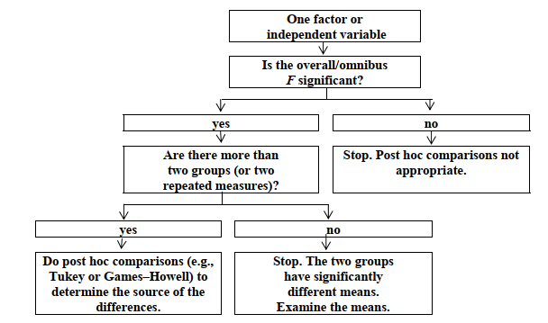
Fig. 10.3. Schematic representation of when to use post hoc multiple comparisons with a one-way ANOVA.

• If the overall F is significant, which pairs of means are significantly different?

After you have examined Output 10.1 to see if the overall F (ANOVA) for each variable was significant, you will do appropriate post hoc multiple comparisons for the statistically significant variables. We will use the Tukey HSD if variances can be assumed to be equal (i.e., the Levene’s test is not significant) and the Games-Howell if the assumption of equal variances cannot be justified (i.e., the Levene’s test is significant).

First we will do the Tukey HSD for grades in h.s. Open the One-Way ANOVA dialog box again by doing the following:

• Select Analyze → Compare Means → One-Way ANOVA… to see Fig. 10.1 again.
• Move visualization test out of the Dependent List: by highlighting it and clicking on the arrow pointing left because the overall F for visualization test was not significant. (See interpretation of Output 10.1.)
• Also move math achievement to the left (out of the Dependent List: box) because the Levene’s test for it was (We will use it later.)
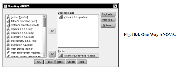
• Keep grades in the Dependent List: because it had a significant ANOVA, and the Levene’s test was not significant.
• Insure that father’s educ revised is in the Factor
• Your window should look like Fig. 10.4.

• Next, click on .. and remove the check for Descriptive and Homogeneity of variance test (in Fig. 10.2) because we do not need to do them again; they would be the same.
• Click on Continue.
• Then, in the main dialogue box (Fig. 10.1), click on Post Hoc. to get Fig. 10.5.
• Check Tukey because, for grades in h.s., the Levene’s test was not significant so we assume that the variances are approximately equal.

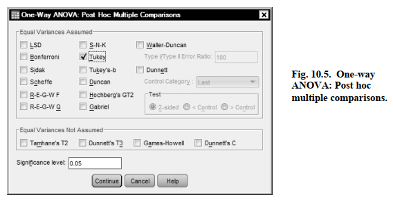
• Click on Continue and then OK to run this post hoc test.

Compare your output to Output 10.2a

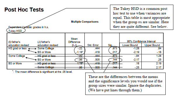
Output 10.2a: Tukey HSD Post Hoc Tests

ONEWAY grades BY faedRevis

/MISSING ANALYSIS

/POSTHOC = TUKEY ALPHA(0.05).

After you do the Tukey test, let’s go back and do Games-Howell. Follow these steps:

• Select Analyze → Compare Means → One-Way ANOVA…
• Move grades in h.s. out of the Dependent List: by highlighting it and clicking on the arrow pointing left.
• Move math achievement into the Dependent List:
• Insure that father’s educ revised is still in the Factor:
• In the main dialogue box (Fig. 10.1), click on Post Hoc. to get Fig. 10.4.
• Check Games-Howell because equal variances cannot be assumed for math achievement.
• Remove the check mark from Tukey.
• Click on Continue and then OK to run this post hoc test.
• Compare your syntax and output to Output 10.2b.

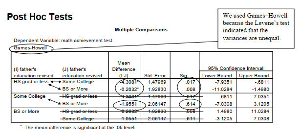
Output 10.2b: Games-Howell Post Hoc Test

ONEWAY mathach BY faedRevis

/MISSING ANALYSIS

/POSTHOC = GH ALPHA(0.05).

Oneway

Interpretation of Output 10.2

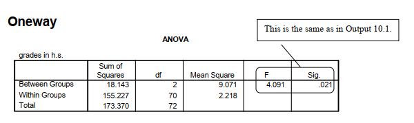
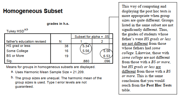
The first table in both Outputs 10.2a and 10.2b repeats appropriate parts of the ANOVA table from Output 10.1. The second table in Output 10.2a shows the Tukey HSD test for grades in h.s. that you would use if the three group sizes (n = 38, 16, 19 from the first table in Output 10.1) had been similar. For grades in h.s., this Tukey table indicates that there is only a small mean difference (.22) between the mean grades of students whose fathers were high school grads or less (M = 5.34 from Output 10.1) and those fathers who had some college (M = 5.56). The Homogeneous Subsets table shows an adjusted Tukey that is appropriate when group sizes are not similar, as in this case. Note that there is not a statistically significant difference (p = .880) between the grades of students whose fathers were high school grads or less (low education) and those with some college (medium education) because their means are both shown in Subset 1. In Subset 2, the medium and high education group means are shown, indicating that they are not significantly different (p = .096). By examining the two subset boxes, we can see that the low education group (M = 5.34) is different from the high education group (M = 6.53) because these two means do not appear in the same subset. Output 10.2b shows, for math achievement, the Games-Howell test, which we use for variables that have unequal variances. Note that each comparison is presented twice. The Mean Difference between students whose fathers were high school grads or less and those with fathers who had some college was -4.31. The Sig. (p = .017) indicates that this is a significant difference. We can also tell that this difference is significant because the confidence interval’s lower and upper bounds both have the same sign, which in this case was a minus, so zero (no difference) is not included in the confidence interval. Similarly, students whose fathers had a B.S. degree were significantly different on math achievement from those whose fathers had a high school degree or less (p = .008).

An Example of How to Write About Outputs 10.1 and 10.2.

Results

A statistically significant difference was found among the three levels of father’s education on grades in high school, F (2, 70) = 4.09, p = .021, and on math achievement, F (2, 70) = 7.88, p = .001. Table 10.2a shows that the mean grade in high school is 5.34 for students whose fathers had low education, 5.56 for students whose fathers attended some college (medium), and 6.53 for students whose fathers received a BS or more (high). Post hoc Tukey HSD tests indicate that the low education group and high education group differed significantly in their grades with a large effect size (p < .05, d = .85). Likewise, there were also significant mean differences on math achievement between the low education and both the medium education group (p < .017, d = .80) and the high education group (p = .008, d = 1.0) using the Games-Howell post hoc test.

Source: Morgan George A, Leech Nancy L., Gloeckner Gene W., Barrett Karen C.

(2012), IBM SPSS for Introductory Statistics: Use and Interpretation, Routledge; 5th edition; download Datasets and Materials.