Analysis of Variance with SPSS – Problem 10.4: Two-Way (or Factorial) ANOVA

In previous problems, we compared two or more groups based on the levels of only one independent variable or factor using t tests (Chapter 9) and one-way ANOVA (this chapter). These were called single factor designs. In this problem, we will compare groups based on two independent variables. The appropriate statistic for this is called a two-way or factorial ANOVA. This statistic is used when there are two different independent variables, each of which classifies (or labels) participants with respect to a particular characteristic, with each participant being labeled by a particular level of each of the independent variables (completely crossed design). For example, an individual could be labeled, or classified, based on the variables of gender and education level, as a female college graduate. In this chapter, we provide an introduction to this complex difference statistic; a more in-depth treatment is provided in Leech et al., in press.

• Do math grades and gender each seem to have an effect on math achievement, and do the effects of math grades on math achievement depend on whether the person is male or female (i.e., on the interaction of math grades with gender)?

Follow these commands:

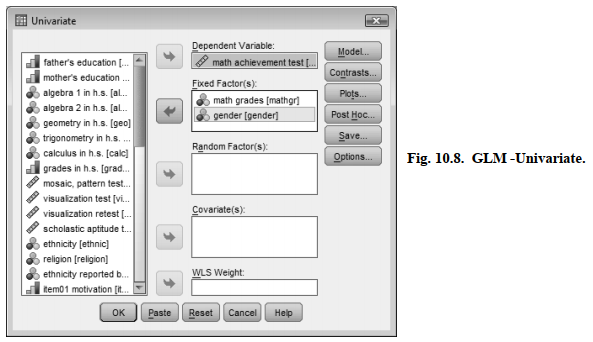
• Analyze → General Linear Model → Univariate…
• Move math achievement to the Dependent Variable:
• Move the first independent variable, math grades (not grades in h.s.), to the Fixed Factor(s):
• Then also move the second independent variable, gender, to the Fixed Factor(s): box (see Fig.10.8)

Now that we know the variables we will be dealing with, let’s determine our options.

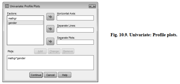
• Click on Plots and move mathgr to the Horizontal Axis: and gender to Separate Lines:
• Then press Add. Your window should now look like Fig. 10.9.
• Click on Continue to get back to Fig. 10.8.

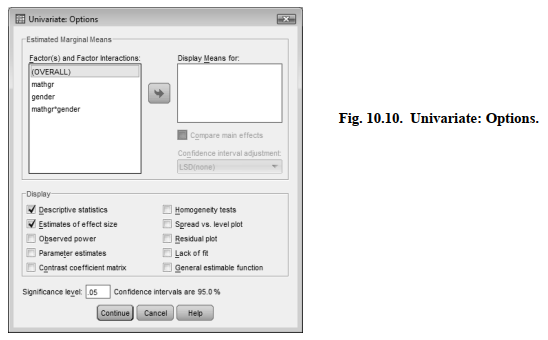
• Select Options and click Descriptive statistics and Estimates of effect size. See Fig. 10.10.
• Click on Continue.
• Click on OK. Compare your syntax and output to Output 10.4.

Output 10.4: Two-Way ANOVA

UNIANOVA mathach BY mathgr gender

/METHOD = SSTYPE(3)

/INTERCEPT = INCLUDE

/PLOT = PROFILE(mathgr*gender )

/PRINT = DESCRIPTIVE ETASQ

/CRITERIA = ALPHA(.05)

/DESIGN = mathgr gender mathgr*gender

Univariate Analysis of Variance

Interpretation of Output 10.4

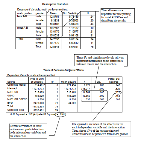
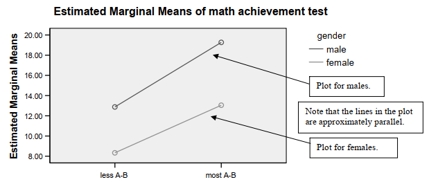
The GLM Univariate program allows you to print the means for each subgroup (cell) representing the interaction between the two independent variables. It also provides measures of effect size (eta²) and plots the interaction, which is helpful in interpreting it. The first table in Output 10.4 shows that 75 participants (44 with less than A-B math grades and 31 mostly A-B math grades) are included in the analysis because they had data on all of the variables. The Descriptive Statistics table shows the cell and marginal (total) means; both are very important for interpreting the ANOVA table and explaining the results of the test for the interaction.

The ANOVA table, called Tests of Between-Subjects Effects, is the key table. Note that the word “effect” in the title of the table can be misleading because this study was not a randomized experiment. Thus, you cannot say in your report that the differences in the dependent variable were caused by or were the effect of the independent variable. Usually you will ignore the lines in the table labeled “corrected model” (which just summarizes all “effects” taken together) and intercept (which is needed to fit the best fit regression line to the data) and skip down to the interaction F (mathgr * gender) which, in this case, is not statistically significant, F (1, 71) = .337, p = .563. If the interaction were significant, we would need to be cautious about the interpretation of the main effects because they could be misleading.

Next we examine the main effects of math grades and of gender. Note that both are statistically significant. The significant F for math grades means that students with fewer As and Bs in math scored lower (M = 10.81 vs. 15.05) on math achievement than those with high math grades, and this difference is statistically significant (p < .001). Gender is also significant (p < .001). Because the interaction is not significant, the “effect” of math grades on math achievement is about the same for both genders. If the interaction were significant, we would say that the “effect” of math grades depended on which gender you were considering. For example, it might be large for boys and small for girls. If the interaction is significant, you should also analyze the differences between cell means (the simple effects). Leech et al. (in press) shows how to do this and discusses more about how to interpret significant interactions. The profile plots may be helpful in visualizing the interaction, but you should not discuss statistically nonsignificant differences because the plots may be misleading.

Note also the callout boxes about the adjusted R squared and eta squared. Eta, the correlation ratio, is used when the independent variable is nominal and the dependent variable (math achievement in this problem) is normal. Eta² is an indicator of the proportion of variance that is due to between-groups differences. Adjusted R² refers to the multiple correlation coefficient squared. Like r², these statistics indicate how much variance or variability in the dependent variable can be predicted if you know the independent variable scores. In this problem, the eta² percentages for these key Fs vary from 0.5% to 17.2%. Because eta and R, like r, are indexes of association, they can be used to interpret the effect size. However, Cohen’s guidelines for small, medium, and large are somewhat different (for eta, small = .10, medium = .24, and large = .37; for R, small = .14, medium = .36, and large = .51).

In this example, eta (not squared) for math grades is about .42 and thus a large effect. Eta for gender is about .40, a large effect. The overall adjusted R is about .46, a large effect. Notice that the adjusted R² is lower than the unadjusted (.22 versus .25). The reason for this is that the adjusted R² takes into account (and adjusts for) the fact that not just one variable but three (math grades, gender, and the interaction) were used to predict math achievement.

An important point to remember is that statistical significance depends heavily on the sample size, so that with 1,000 subjects a much lower F or r will be significant than if the sample is 10 or even 100. Statistical significance just tells you that you can be quite sure that there is at least a little relationship between the independent and dependent variables. Effect size measures, which are more independent of sample size, tell you how strong the relationship is and thus give you some indication of its importance.

The profile plots of cell means (which follow the table of between-subjects effects) help us to visualize the nature of a significant interaction when one exists. When the lines on the profile plot are parallel, there is not a significant interaction. Note that we requested that the separate lines represent the two genders because we felt that this would make a significant interaction easier to interpret than if the two lines represented predominant level of grades. However, really, either independent variable could have been represented in either part of the graph.

An Example of How to Write About Output 10.4

Results

To assess whether math grades and gender each seem to have an effect on math achievement, and if the effects of math grades on math achievement depend on whether the person is male or female (i.e., on the interaction of math grades with gender) a two-way ANOVA was conducted.

Table 10.4a shows the means and standard deviations for math achievement for the two genders and math grades groups. Table 10.4b shows that there was not a significant interaction between gender and math grades on math achievement (p = .563). There was, however, a significant main effect of gender on math achievement, F (1, 71) = 13.87, p < .001. Eta for gender was about .42, which, according to Cohen (1988), is a large effect. Furthermore, there was a significant main effect of math grades on math achievement, F (1, 71) = 14.77, p < .001. Eta for math grades was about .40, a large effect.

Source: Morgan George A, Leech Nancy L., Gloeckner Gene W., Barrett Karen C.

(2012), IBM SPSS for Introductory Statistics: Use and Interpretation, Routledge; 5th edition; download Datasets and Materials.