This section puts the principal methods into practice. We recommend researchers seeking a more detailed discussion of the practical application of these structuring and classifying methods refer to a specialized data analysis manual, such as Hair et al. (1992).
1. Cluster Analysis
After clearly defining the environment from which the objects to be classified have been drawn, and then preparing the data appropriately, a researcher who undertakes to conduct a cluster analysis must choose a classification algorithm, determine the number of classes necessary and then validate them.
1.1. Choosing a classification algorithm
Choosing a classification algorithm involves deciding which procedure, hierarchical or non-hierarchical, to use in order to correctly group discrete objects into classes.
Several classification algorithms exist. Two different types of procedure are commonly distinguished: hierarchical procedures and non-hierarchical procedures.
Hierarchical procedures break down a database into classes that fit one inside the other in a hierarchical structure. These procedures can be carried out in an agglomerative or a divisive manner. The agglomerative method is the most widely used. From the start, each object constitutes a class in itself. The first classes are obtained by grouping together those objects that are the most alike. The classes that are the most alike are then grouped together – and the method is continued until only one single class remains. The divisive method proceeds by successive divisions, going from classes of objects to individual objects. At the start, all of the objects constitute a single class – this is then divided to form two classes, which are as heterogeneous as possible. The procedure is repeated until there are as many classes as there are different objects.
Several hierarchical classification algorithms exist. The Ward algorithm is the most often used in management research, as it favors the composition of classes of the same size. For a more in-depth discussion of the advantages and limits of each algorithm, the researcher can consult specialist statistical works, different software manuals (SAS, SPSS, SPAD, etc.), or articles that present meta-analyses of algorithms used in management research (Ketchen and Shook, 1996).
Non-hierarchical procedures – often referred to as K-means methods or iterative methods – involve groupings or divisions which do not fit one inside the other hierarchically. After having fixed the number (K) of classes he or she wishes to obtain, the researcher can, for each of the K classes, select one or several typical members – ‘core members’ – to input into the program.
Each of these two approaches has its strengths and its weaknesses. Hierarchical methods are criticized for being very sensitive to the environment from which the objects that are to be classified have been drawn, to the preparatory processing applied to the data (to allow for outliers and missing values, and to standardize variables) and to the method chosen to measure proximity. They are also criticized for being particularly prone to producing classes which do not correspond to reality. Non-hierarchical methods are criticized for relying completely on the subjectivity of the researcher who selects the core members of the classes. Such methods demand, meanwhile, good prior knowledge of the environment from which the objects being classified have been drawn; which is not necessarily the case in exploratory research. However, non-hierarchical methods are praised for not being over-sensitive to problems linked to the environment of the objects being analyzed – in particular, to the existence of outliers.
In the past, hierarchical methods were used very frequently, certainly in part for reasons of opportunity: for a long time these methods were the most well documented and the most readily available. Non-hierarchical methods have since become more accepted and more widespread. The choice of algorithm depends, in the end, on the researcher’s explicit or implicit hypotheses, on his or her degree of familiarity with the empirical context and on the prior existence of a relevant theory or published work.
Several specialists advise a systematic combination of the two types of methods (Punj and Steward, 1983). A hierarchical analysis can be conducted initially, to obtain an idea of the number of classes necessary, and to identify the profile of the classes and any outliers. A non-hierarchical analysis using the information resulting from hierarchical analysis (that is, number and composition of the classes) then allows the classification to be refined with adjustments, iterations and reassignments within and across the classes. This double procedure increases the validity of the classification (see Section 2, subsection 1.3 in this chapter).
1.2. Number of classes
Determining the number of classes is a delicate step that is fundamental to the classification process. For non-hierarchical procedures, the number of classes must be established by the researcher in advance – whereas for hierarchical procedures it is deduced from the results. While no strict rule exists to help researchers determine the ‘true’ or ‘right’ number of classes, several useful criteria and techniques are available to them (Hardy, 1994; Moliere, 1986; Ohsumi, 1988).
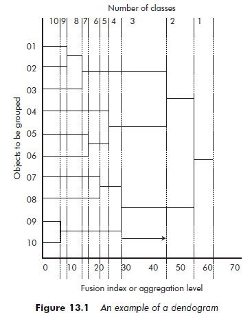
Virtually all hierarchical classification software programs generate graphic representations of the succession of groupings produced. These graphs – called dendograms – consist of two elements: the hierarchical tree and the fusion index or agglomeration coefficient. The hierarchical tree is a diagrammatic reproduction of the classified objects. The fusion index or agglomeration coefficient is a scale indicating the level to which the agglomerations are effected. The higher the fusion index or agglomeration coefficient, the more heterogeneous the classes formed.
Figure 13.1 shows an example of a dendogram. We can see that the objects that are the closest, and are the first to be grouped together, are objects 09 and 10. Aggregations then occur reasonable regularly, without any sudden rises, until the number of classes has been reduced to three. However, when we pass from three classes to two (see arrow on Figure 13.2), there is a big ‘leap’ in the fusion index (see the arrow on the graph). The conclusion is that three classes should be kept.
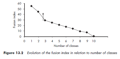
The researcher may be faced with situations where there is no visible leap in the fusion index, or where there are several. The first situation may signify that there are not really any classes in the data. The second signifies that several class structures are possible.
Finally, another often used criterion is the CCC (Cubic Clustering Criterion). This is a means of relating intra-class homogeneity to inter-class heterogeneity. Its value for each agglomeration coefficient (that is, each number of classes) is produced automatically by most automatic classification software programs. The number of classes to use is the number for which the CCC reaches a maximum value – a ‘peak’. Several researchers have used this criterion (Ketchen and Shook, 1996).
1.3. Validating the classes
The final step in using cluster analyses is to verify the validity of the classes obtained. The aim is to ensure the classification has sufficient internal and external validity (the concept of validity is presented in detail in Chapter 10). In the case of cluster analyses, there are three important aspects to consider: reliability, predictive validity and external validity.
The reliability of the instruments used can be evaluated in several ways. The researcher can apply different algorithms and proximity measurements then compare the results obtained. If the classes highlighted remain the same, the classification is reliable (Hair et al., 1992; Ketchen and Shook, 1996; Lebart et al., 1984). Equally, one can divide a sufficiently large database into two parts and carry out the procedures on each of the separate parts. Concordance of the results is an indication of their reliability. Hambrick’s (1983) research on mature industrial environments is a good example of this method.
Predictive validity should always be examined in relation to an existing conceptual base. Thus, the many authors who have used cluster analyses to identify strategic groups would be able to measure the predictive validity of their classifications by studying the relationship between the classes they obtained (that is, the strategic groups) and performance. In fact, the strategic groups theory stipulates that membership of a strategic group has a determining influence on performance (Porter, 1980). If a classification enables us to predict performance, it has a good predictive validity.
There are no tests specifically designed to test the external validity of cluster analyses. One can still, however, appreciate the quality of the classification by carrying out traditional statistical tests (Fisher’s F, for example) or analyses of the variance between the classes and external measurements. For example, a researcher may set about classifying industrial supply firms and find two classes; that of the equipment suppliers and that of the subcontractors. To test the validity of his or her typology, the researcher may carry out a statistical test on the classes obtained and on a variable not taken into account in the typology. If the test is significant, he or she will have strengthened the validity of the classification. If the reverse occurs, he or she will need to examine the reasons for this non-validation. The researcher could question, for instance, whether the external measurement he or she has chosen is suitable, whether there are errors in his or her interpretation of the classes and whether the algorithms he or she has chosen are consistent with the nature of the variables and his or her research method.
The external validity of a classification can also be tested by carrying out the same analysis on another database and comparing the results obtained (Hair et al., 1992). This method is difficult to use in most research designs in management, however, as primary databases are often small and it is not easy to access complementary data. It is rarely possible to divide the data into different sample groups. Nevertheless, this remains possible when the researcher is working with large secondary databases.
1.4. Conditions and limitations
There are numerous possible ways cluster analyses can be useful research tools. Not only are they fundamental to studies aimed at classifying data, but they are also regularly used to investigate data, because they can be applied to all kinds of data.
In theory, we can classify everything. But while this may be so, researchers should give serious thought to the logic of their classification strategies. They must always consider the environmental homogeneity of the objects to be classified, and the reasons for the existence of natural classes within this environment – and what these may signify.
The subjectivity of the researcher greatly influences cluster analysis, and represents one of its major limitations. Even though there are a number of criteria and techniques available to assist researchers in determining the number of classes to employ, the decision remains essentially up to the researcher alone.
Justification is easier when these classes are well defined, but in many cases, class boundaries are less than clear-cut, and less than natural.
In fact, cluster analysis carries a double risk. A researcher may attempt to divide a logical continuum into classes. This is a criticism that has been leveled at empirical studies that attempt to use cluster analysis to validate the existence of the two modes of governance (hierarchical and market) proposed by Williamson. Conversely, the researcher may be attempting to force together objects that are very isolated and different from each other. This criticism is sometimes leveled at works on strategic groups which systematically group firms together (Barney and Hoskisson, 1990).
The limitations of classification methods vary according to the researcher’s objectives. These limitations are less pronounced when researchers seek only to explore their data than when their aim is to find true object classes.
2. Factor Analysis
Factor analysis essentially involves three steps: choosing an analysis algorithm, determining the number of factors and validating the factors obtained.
2.1. Choosing a factor analysis technique
Component analysis and common and specific factors analysis There are two basic factor analysis techniques (Hair et al., 1992): ‘classic’ factor analysis, also called common and specific factor analysis, or CSFA, and component analysis, or CA. In choosing between the two approaches, the researcher should remember that, in the framework of factor analysis, the total variance of a variable is expressed in three parts: (1) common, (2) specific and (3) error. Common variance describes what the variable shares with the other analysis variables. Specific variance relates to the one variable in question. The element of error comes from the imperfect reliability of the measurements or to random component in the variable measured.
In a CSFA, only common variance is taken into account. The variables observed, therefore, are the linear combinations of non-observed factors, also called latent variables. Component analysis, on the other hand, takes total variance into account (that is, all three types of variance). In this case it is the ‘factors’ obtained that are linear combinations of the observed variables. The choice between CSFA and CA methods depends essentially on the researcher’s objectives. If the aim is simply to summarize the data, then CA is the best choice. However, if the aim is to highlight a structure underlying the data (that is, to identify latent variables or constructs) then CSFA is the obvious choice. Both methods are very easy to use and are available in all major software packages.
Correspondence factor analysis A third, albeit less common, type of factor analysis is also possible: correspondence factor analysis (Greenacre, 1993;
Greenacre and Blasius, 1994; Lebart and Mirkin, 1993). This method is used only when a data set contains categorical variables (that is, nominal or ordinal). Correspondence factor analysis was invented in France and popularized by Jean-Paul Benzecri’s team (Benzecri, 1992). Technically, correspondence factor analysis is similar to conducting a CA on a table derived from a categorical database. This table is derived directly from the initial database using correspondence factor analysis software. However, before beginning a correspondence factor analysis, the researcher has to categorize any metric variables present in the initial database. An example of such categorization is the transformation of a metric variable such as ‘size of a firm’s workforce’ into a categorical variable, with the modalities ‘small’, ‘medium’ and ‘large’. All metric variables can be transformed into a categorical variable.
Otherwise, aside from the restriction of it being solely applicable to the analysis of categorical variables, correspondence factor analysis is subject to the same constraints and same operating principles as other types of factor analysis.
2.2. Number of factors
Determining the number of factors is a delicate step in the structuring process. While again there is no general rule for determining the ‘right’ number of factors, a number of criteria are available to assist the researcher in approaching this problem (Stewart, 1981). We can cite the following criteria:
A priori specification’ This refers to situations when the researcher already knows how many factors need to be included. This approach is relevant when the research is aimed at testing a theory or hypothesis relative to the number of factors involved, or when the researcher is replicating earlier research and wishes to extract exactly the same number of factors.
‘Minimum restitution’ The researcher fixes in advance a level corresponding to the minimum percentage of information (that is, of variance) that is to be conveyed by all of the factors retained (for example, 60 per cent). While in the exact sciences, percentages of 95 per cent are frequently required, in management percentages of 50 per cent and even much lower are often considered satisfactory (Hair et al., 1992).
The Kaiser rule According to the Kaiser rule, the researcher includes only those factors whose eigenvalues (calculated automatically by computer software) are greater than one. The Kaiser rule is frequently applied in management science research – although it is only valid without restrictions in the case of a CA carried out on a correlation matrix. In the case of a CSFA, the Kaiser rule is too strict. According to this rule, the researcher can retain a factor whose eigenvalue is less than one, as long as this value is greater than the mean of the variables’ communalites (common variances). This rule gives the most reliable results for cases including from 20 to 50 variables. Below 20 variables, it tends to reduce the number of factors, and above 50 variables, to increase it.
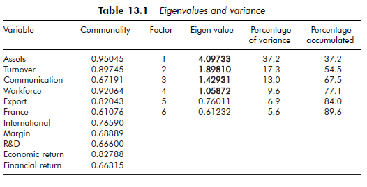
Example: Factors and associated eigenvalues
Table 13.1 presents the results of a factor analysis. Eleven variables characterizing 40 firms were used in the analysis. For each variable, communality represents the share of common variance. The first six factors are examined in the example. According to the Kaiser rule, only the first four factors must be retained (they have an eigenvalue of more than 1). In total, these first four factors reproduce 77.1 per cent of the total variance.
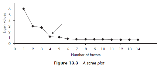
The eigenvalues are classified in decreasing order and any definite leveling- out of the curve is noted. The number of factors to include is then the number corresponding to the point where this leveling-out begins. Factor analysis software packages can generate a graphic visualization – called a ‘scree plot’ or a ‘scree test’ – of eigenvalues, which facilitates detection of such leveling. Figure 13.3 shows an example of a ‘scree plot’. It represents the eigenvalues of the first 14 factors resulting from a CA. We note that, after the fourth factor, the eigenvalues stabilize (see arrow on Figure 13.3). The number of factors to retain is, therefore, four.
Factor interpretation is at the heart of factor analysis; notably CSFA, where it is often important to understand and sometimes to name the latent variables (that is, the factors). One frequently used technique is rotation. Rotation is an operation that simplifies the structure of the factors. Ideally, each factor would load with only a small number of variables and each variable would load with only a small number of factors, preferably just one. This would enable easy differentiation of the factors. A distinction needs to be made between orthogonal rotations and oblique rotations. In an orthogonal rotation, the factors remain orthogonal in relation to each other while, in an oblique rotation, this constraint is removed and the factors can load with each other. The rotation operation consists of two steps. First, a CA or a CSFA is carried out. On the basis of the previously mentioned criteria, the researcher chooses the number of factors to retain; for example, two. Rotation is then applied to these factors. We can cite three principal types of orthogonal rotation: Varimax, Quartimax and Equamax.
The most widespread method is Varimax, which seeks to minimize the number of variables strongly loaded with a given factor. For each factor, variable correlations (factor loading) approach either one or zero. Such a structure generally facilitates interpretation of the factors, and Varimax seems to be the method that gives the best results. The Quartimax method aims to facilitate the interpretation of the variables by making each one strongly load with one factor, and load as little as possible with all the other factors. This means that several variables can be strongly loaded with the same factor. In this case, we obtain a kind of general factor linked to all the variables. This is one of the main defects of the Quartimax method. The Equamax method is a compromise between Varimax and Quartimax. It attempts to somewhat simplify both factors and variables, but does not give very incisive results and remains little used. Oblique rotations are also possible, although these are given different names depending on the software used (for example, Oblimin on SPSS or Promax on SAS). Oblique rotations generally give better results than orthogonal rotations.
To interpret the factors, the researcher must decide on which variables are significantly loaded with each factor. As a rule, a loading greater than 0.30 in absolute value is judged to be significant and one greater than 0.50 very significant. However, these values must be adjusted in relation to the size of the sample, the number of variables and factors retained. Fortunately, many software packages automatically indicate which variables are significant.
Example: Matrix, rotations and interpretation of the factors
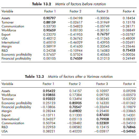
Tables 13.2 and 13.3 follow from the factor analysis results presented above in Table 13.1. These tables reproduce the standard output of factor analysis software. We should remember that the first four factors were retained according to the Kaiser rule (eigenvalue greater than one). Table 13.2 presents the matrix of the factors before rotation. One can conclude that the variables ‘assets’, ‘workforce’ and ‘turnover’ are strongly and essentially loaded to Factor 1 and that the variable ‘financial profitability’ is strongly and essentially loaded to Factor 2. However, the other variables are strongly loaded to several factors at once. Such a situation makes interpretation relatively difficult. It can, therefore, be useful to proceed to a factor rotation.
Table 13.3 presents the matrix of factors after a Varimax rotation. One can conclude that the variables ‘assets’, ‘workforce’ and ‘turnover’ are always strongly and essentially loaded to Factor 1. The variables ‘economic profitability’, ‘financial profitability’ and ‘margin’ seem to be strongly and essentially loaded to Factor 2. The variables ‘export’ and ‘international’ as well as, to a lesser degree, the variable ‘communication’, are strongly and essentially loaded to Factor 3. Finally, the variable ‘R&D’ and, to a lesser degree, the variable ‘USA’ are strongly and essentially loaded to Factor 4. In conclusion, the interpretation of the factors is simplified: Factor 1 represents ‘size’, Factor 2 ‘profitability’, Factor 3 ‘internationalization policy’ and Factor 4 ‘research and development policy’.
2.3. Validation
The final step in a factor analysis involves examining the validity of the factors obtained. The same methods that may be applied to increase the reliability of cluster analyses (that is, cross-correlating algorithms, dividing a database) can also be used for factor analyses.
Factor analyses are often aimed at identifying latent dimensions (that is, variables that are not directly observable) that are said to influence other variables. In strategic management, for example, numerous ‘factors’ have been found to influence the performance of companies. These include strategy, organizational structure, planning, information and decision-making systems. Researchers wanting to operationalize such factors (that is, latent variables) could study the predictive validity of the operationalizations obtained. For example, researchers who undertake to operationalize the three ‘generic strategies’ popularized by Porter (1980) – overall low cost, differentiation and focus – would then be able to examine the predictive validity of these three factors by evaluating their relationship to the firms’ performances.
Researchers can test the external validity of their factor solutions by replicating their study in another context or with another data set. That said, in most cases it would not be possible for the researcher to access a second empirical context. The study of external validity can never simply be a mechanical operation. A thorough preliminary consideration on the content of the data to be analyzed, as developed in the first section of this chapter, can provide a good basis for studying the external validity of a factor analysis.
2.4. Conditions and limitations
Factor analysis is a very flexible tool, with several possible uses. It can be applied to all kinds of objects (observations or variables) in various forms (tables of metric or categorical data, distance matrices, similarity matrices, contingency and Burt tables, etc.).
As with cluster analyses, the use of factor analysis entails a certain number of implicit hypotheses relating to the environment of the objects to be structured. Naturally, there is no reason why the factors identified should necessarily exist in a given environment. Researchers wishing to proceed to a factor analysis must, therefore, question the bases – theoretical or otherwise – for the existence of a factor structure in the particular environment of the objects to be structured. Most factor analysis software automatically furnishes indicators through which the probability of a factor structure existing can be determined and the quality of the factor analysis assessed. Low quality is an indication of the absence of a factor structure or the non-relevance of the factorial solution used by the researcher.
Finally, it must be noted that the limitations of factor analysis vary depending on the researcher’s objectives. Researchers wishing simply to explore or synthesize data have much greater freedom than those who propose to find or to construct underlying factors.
Source: Thietart Raymond-Alain et al. (2001), Doing Management Research: A Comprehensive Guide, SAGE Publications Ltd; 1 edition.
Great article.
Amazing! Its truly awesome post, I have got much clear idea on the topic of from this piece of writing.