Capital structure and corporate governance of the firm

1. The Modigliani-Miller Theorem

Throughout this chapter the agency problems of corporate control have been to the fore. Yet, although financial instruments such as ordinary shares and various types of debt have been mentioned and the conse­quences for incentives have been noted, we have not linked observed finan­cial structure systematically to control problems. The question of what determines the capital structure of firms now comprises a substantial part of modern financial theory and the reader is referred to a specialised text for a more extensive treatment.²² It is important to sketch the outlines of the subject, however, because the financial structure of a modern corpora­tion can be seen as a response to some of the agency problems that we have been discussing.

Just as traditional neoclassical theory provided no satisfactory rational­isation of firms, the neoclassical theory of finance had little to say about the choice of financial structure. In a pathbreaking contribution to the theory of finance, for example, Modigliani and Miller (1958) showed that, under conditions of full information, the value of the firm would be inde­pendent of the means chosen to finance it. The debt-equity ratio would not influence the value of the firm.²³ The Modigliani-Miller theorem provides the same sort of benchmark in finance as the work of Ronald Coase pro­vides in the theory of economic organisation (see, again, Chapter 2). With no transactions costs and full public information, organisational structure would be indeterminate because there is no organisational problem to solve. Similarly, with costless and perfect markets, the means of finance is irrelevant to the firm’s valuation and there is no particular ‘optimal’ finan­cial structure.

The Modigliani-Miller theorem seems, at first acquaintance, counterin­tuitive. There appears to be a deceptive implication that the riskiness of an asset will not influence its price. This, however, would be a complete mis­interpretation. The theorem does not tell us that the market value of firms is independent of the risk and return characteristics of their anticipated net cash flows. On the contrary, the theorem asserts that it is precisely the nature of these anticipated cash flows that will determine the value of the firm and not the nature of the financial instruments issued by the firm to lay claim to them.

Consider two firms setting out the various ‘states of nature’ that might happen in the future and calculating the net cash flows that they would receive were those states of nature to materialise. Suppose the firms are identical except that one is financed entirely by equity while the other is financed with both equity and debt. Assume that the debt is risk free and that in neither firm does bankruptcy occur in any state of nature. The total market value of the outstanding claims must be the same for each firm. If this were not the case and the shares of the all-equity firm were valued, in total, more highly than the shares plus bonds of the firm with both equity and debt, profitable arbitrage possibilities would exist for holders of the securities. If, for example, a person held one hundred per cent of the shares of the all-equity firm, he or she would sell them and buy the shares plus bonds of the other firm. The claims to net cash flow represented by the mixed portfolio are (by assumption) the same overall as the claims repre­sented by the all-equity portfolio. Thus, the market prices of stocks and bonds will so adjust that firms with the same risk and return characteristics will have the same total market valuation, irrespective of their financial structure.

Similar types of argument can also be used to show that the firm’s policy on distributions will not affect its value. Whether a firm retains its earnings to invest in a project or distributes earnings and raises funds by issuing new equity, will not matter. In the former case, share prices will rise to reflect higher future cash flows from the investment. In the latter case, the greater value of the firm will be reflected in a larger number of outstanding shares. Individual shareholders will not be affected because they can always adjust their own portfolio of shares to neutralise the actions of the firm. If the firm finances an investment by retentions, for example, a shareholder who is unwilling to contribute can simply sell sufficient of his or her shares to offset the rise in their total value.

It is evident that a theory which explains the financial structure of firms cannot be based upon assumptions of costless and frictionless markets with full information. The final paragraphs of this section aim to describe how the information and agency problems discussed earlier relate to the choice of financial structure. As we have seen, moral hazard and adverse selection problems deriving from asymmetric information are at the centre of the stage. In addition, however, bounded rationality and the incomplete and imperfectly specified nature of contracts play an important part.

2. The Agency Costs Theory of Financial Structure

A formal analysis of the incentive problems associated with joint-stock enterprise is presented by Jensen and Meckling (1976). Their approach incorporates the use of debt instruments as well as equity in a sophisticated theory of ‘ownership structure’. At this point we merely outline the sim­plest case, and consider the effect of outside-equity holders on the market value of the firm. Suppose that the firm is of a given size, that it is financed entirely by equity and that initially all the equity is held by a single manager or ‘peak coordinator’. In Figure 9.1, the market value of the firm is meas­ured on the vertical axis and the market value of the stream of ‘expendi­tures on non-pecuniary benefits’ is measured along the horizontal axis. The slope of the constraint VF is — 1, indicating that expenditures on non­pecuniary benefits are at the expense of pecuniary benefits. A single pro­prietor will operate at point a, where his or her indifference curve U₁ is tangential to the constraint VF. The market value of the firm as a single proprietorship will be OV*, and the non-pecuniary benefits available will have a value of OF*.

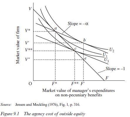
Now assume that the ‘peak coordinator’ can sell a fraction of his or her equity shares to outsiders. These shares, Jensen and Meckling assume, carry no voting rights. Suppose that the peak coordinator retains a proportion of the shares and sells a proportion 1 -α. Clearly the ‘cost’ to the coordinator of ‘managerial’ expenditures on non-pecuniary benefits will now only be a fraction a of the reduction in the market value of the firm which results. We would therefore expect the peak coordinator to indulge in more ‘man­agerial’ expenditures than before, and the market value of the equity shares will fall. This change in behaviour induced by the manager’s smaller pro­portionate stake in the enterprise will be predicted by the outsiders who purchase equity from him/her and they will adjust downwards the price they are prepared to pay for the shares accordingly. An outside investor short-sighted enough to pay (1 – α) V* for the shares offered would suffer a loss. The peak coordinator would not remain at point a with wealth V* (made up of (1 – α) V* in cash and a V* of remaining equity) and with man­agerial perks of OF*. S/he would increase his/her nonpecuniary expendi­tures to OF and his/her private wealth would fall to O V’. The value of the firm would fall precipitously to O V”, but a fraction (1 – α) of this fall would be borne by the outsider, not the manager.

When the outsider purchases a fraction 1—α of the equity, s/he will revise downwards the value of the firm to OK**. Assuming the outsider’s expectations about managerial shirking are correct, the manager will operate at point c in Figure 9.1. The total value of the firm’s equity will be O K** and the manager will indulge in OF** of non-pecuniary benefits. Any higher initial valuation of the shares would result in the outsiders making a loss as already described, and any lower valuation would imply that the peak coordinator had sold for less than outsiders would have been prepared to pay. The distance OK* — OK** is termed by Jensen and Meckling the gross agency cost of the move to a fraction 1—a of outside equity. We should note that this fall in the value of the firm would not occur if an enforceable contract could be drawn up limiting the manager’s non­pecuniary benefits to OF*. Thus, even where monitoring is costly, some arrangement of this type might be in the interests of both parties.

If outside equity reduces the value of the firm and results in ‘agency costs’, why is it that all firms are not individually owned and managed? One answer might be that no single individual is wealthy enough to hold the entire equity. This does not, however, explain why, if this is so, capital could not be borrowed at fixed interest instead of raised by outside equity holders. The objection that proprietors would not like highly leveraged operations because of the risk of bankruptcy has less force in a world of limited liabil­ity than one of unlimited liability. Under limited liability, the problem is not the risk aversion of the owner-manager but instead the incentives that a highly leveraged structure will give to such a person to take very large risks. The costs of failure are borne by outside bondholders and the benefits of success go to the single equity holder. Clearly, there are agency costs asso­ciated with the use of debt as well as outside equity.

Given the inescapable agency costs of outside finance, Jensen and Meckling explain the existence of outside equity and debt holders primar­ily by reference to risk-spreading benefits. Selling equity claims to outsid­ers will reduce the value of the firm and hence the owner-manager’s wealth, but if the benefits of a more widely diversified portfolio outweigh these agency costs, the owner-manager will still prefer to reduce his/her holding. The optimal amount of outside financing will be reached when the margi­nal benefits from increased diversification equal the marginal agency costs incurred.²⁴

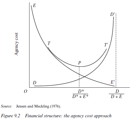
Figure 9.2 summarises the agency costs approach to capital structure. Let E be outside equity and D represent the issue of debt. Along the hori­zontal axis, the proportion of equity finance declines and the proportion of debt finance increases. We have seen that as the proportion of outside equity increases, managerial effort declines and gross agency costs of equity rise. This relationship is represented by the curve labelled EE’ in Figure 9.2.

Similarly, as the proportion of bond finance rises and outside equity declines, the agency problems of debt become increasingly serious. Inside- equity holders have greater effort incentives, and bond finance ensures the distribution of cash from successful ventures, but bonds also encourage greater risk taking. This relationship is shown by curve DD’. Total agency costs are minimised at point P on TT.

3. Agency Problems, Debt and the Hart-Moore Theory of Financial Structure

3.1. Non-contractibility and financial structure

In section 10.2, the use of debt was seen as constrained by the potential opportunistic behaviour of a few significant equity holders. Jensen and Meckling’s theory therefore applies to situations in which owner-managers hold all the control rights and a significant portion of profit rights. In this subsection, agency problems remain to the fore, but we return to the main focus of Chapters 8 and 9 – the problem of controlling managers who may have negligible profit rights. In a modern joint-stock enterprise, we take it as given that equity holdings are widely dispersed, that incentive contracts will not always align managerial interests with those of shareholders and that managers therefore have considerable scope to indulge in discretionary behaviour. Debt instruments can then be seen as the means by which the diversion of resources towards managerial ends is controlled. Hart and Moore (1995) have developed this theory, which extends the type of reason­ing explored in Chapter 4, subsection 8.2, on the finance of the entrepren­eur. There, the contract of debt was a means of forcing the entrepreneur to disgorge revenue flows when these were assumed not to be ex ante contract­ible. Here, short-term debt can be seen similarly as a mechanism for forcing managers to distribute cash flows rather than wasting them on unprofitable projects.²⁶ Short-term debt also forces managers to liquidate investments when this is better than pursuing them further at a loss. Long-term debt can likewise be seen as a mechanism for preventing managers from undertak­ing loss-making new ventures, whilst permitting them to continue with profitable existing ones.

Suppose, adjusting the exposition of Chapter 4, that a project under­taken at the beginning of period 1 yields revenues of R₁ and R₂ at the end of periods 1 and 2 respectively. The liquidation value of the project at the end of period 1 is K₁. In the context of this chapter, the project is under­taken not by an entrepreneur but a ‘manager’. The revenue stream is still not contractible because not verifiable but, unlike the model introduced in Chapter 4, we do not assume that the manager can simply steal these reve­nues and divert them to his or her own purposes. Instead, we assume that the manager gets private benefits from undertaking projects whether or not they are profitable. Revenue streams and cash flows from liquidation are received by outside equity holders or the holders of short- or long-term debt. For simplicity, the rate of discount is assumed to be zero.

3.2. Short-term debt and project liquidation

Financial structure, in this model, is about constraining managers. Clearly, if R₂ < K₁, it is efficient to liquidate the project at the end of period 1. Managerial interests, however, dictate that the project should go on if it can possibly be arranged. Managers cannot be controlled directly by the owners and told to liquidate such a project, because owners are dispersed and because a suitable contract to this end cannot be written. Short-term debt can be used in this situation to force liquidation. Suppose that the manager must make a payment to bond holders at the end of period 1 of P₁. A suffi­ciently large value of P₁ will force the manager either to liquidate the assets or to borrow sufficient new funds to permit the project to continue. In par­ticular, if P₁ > R₁, the manager will have to default unless new borrowing can be arranged. Will the manager be able to borrow P₁ – R₁ so as to avoid defaulting on the short-term debt? Assume for the time being that there is no outstanding long-term debt with its associated obligations to repay at the end of period 2. Managers will be able to raise new finance, providing R₂ > P_J -Rj. To prevent this happening, owners must set P_J > R_J +R₂.

If revenue flows are known with certainty at the beginning of period J, therefore, sufficiently high levels of short-term debt can force liquidation at the end of period J, if this is efficient. Bond holders would receive P_J while equity holders would receive R_J + K_J — P_J. Given that we are assuming that K_J >R₂, it is possible for equity to receive a positive return under these circumstances. The problem, of course, is that revenues are not known with certainty at the beginning of period J. If we make the assumption that it is only at the end of period J that managers and providers of finance will know whether or not the project should be liquidated or continued into period 2, the dangers of high levels of short-period debt become apparent. The managers might be forced into liquidation even if it transpired that K_J < R₂ and the project should continue. To avoid inefficient liquidation, a low level of short-term debt is required. If we knew with certainty that K_J < R₂ and that the project should continue, we could set P_J = 0 and there would be no role for short-term debt.

Suppose now that there are two possible scenarios for the outcome of the project (scenario A and scenario B). Which scenario prevails will not be known until the end of period J. If both scenarios involve keeping the project going to the end of period 2, it is easy to see that P_J = 0 is the best solution for short-term debt. Similarly, if the project should be liquidated at the end of period J under both scenarios, a sufficiently high level of P_J will be able to accomplish this. The more interesting cases involve R₂^A > K_J^A and R₂^b<K_J^B. In other words, it would be best to continue to the end of period 2 under scenario A, but liquidate the project at the end of period J under scenario B. Is there a level of P_J which will force closure under sce­nario B and permit continuation under scenario A?

There are several possibilities to consider. Suppose first that revenue in period J is higher in scenario A than scenario B (R_J^A> R_J^B). This implies that we can set the level of short-term debt (say) P* below R_J^A and above R_J^B, thereby posing no financing problem to the managers at the end of period J in scenario A while forcing them to seek new borrowing in scenario B. How, though, can we be sure that the managers in scenario B will not find willing lenders? Clearly, they might do so if revenue at the end of period 2 exceeds the level of borrowing necessary to keep going (R₂^B> P* — R_J^B) and this possibility is not ruled out by any of our assumptions. One way of preventing the managers successfully finding finance to continue the project inefficiently in scenario B is to issue senior long-term debt repayable at the end of period 2, or before if the project is liquidated. Potential lenders at the end of period J will observe that there are already prior claimants to some of next period’s revenue. They will lend only if R₂^B>P_J + P₂ — R_J^B, where P₂ is the level of long-term debt obligations. While P_j is constrained to be no higher than R₁^A, so that there are no impediments to continuing the project in scenario A, there are no such limitations on the level of P₂. The level of long-term senior debt can therefore be set at a level sufficient to prevent managers in scenario B extending the life of the project ineffi­ciently.

What happens, however, if scenario A’s revenue is lower than scenario B’s in period 1 (R₁^A < R₁^B)? Setting the level of P_j low enough not to inconven­ience managers in scenario A will imply that it is also low enough to leave them unhindered in scenario B. If we are to control managerial behaviour in scenario B, we cannot avoid forcing the managers into the financial markets in both scenarios. This will not matter, providing the managers can successfully find the necessary finance to continue under A but are forced to liquidate under B. Thus, if R₂^A >P_J – R₁^A but R₂^B < P_j – R₁^B, managers can find finance under A but not under B. These conditions can be satisfied if R₁^A + R₂^a > R₁^B+R₂^b. The level of short-term debt (say P_j*) can be set below the present value of revenues in scenario A but above the present value of revenues in scenario B. This forces liquidation under B but not under A, as required.

The real problem case is where the present value of revenues under sce­nario B exceeds that under A, even though it is under B that the project should be liquidated at the end of the first period (R₁^A + R₂^A<R₁^B+R₂^B). Setting P_j between the present value of revenue streams would simply force managers to liquidate the project under A but not under B – the reverse of what is required. The choice is therefore either to liquidate the project under both scenarios using a high value of P_j or to continue it under both with P* = 0. Clearly, the best policy will depend upon the probabilities attached to scenarios A and B respectively. The higher the probability of scenario A, the more likely it is that we will want the project to continue and the better it will be to opt for low levels of short-term debt. The greater the probabil­ity of scenario B, the more likely that we will wish to liquidate the project and the better it will be to opt for high levels of short-term debt.

3.3. Long-term debt and new investment

We have already noticed in subsection 10.3.2 that, under certain circum­stances, the existence of long-term debt obligations might prevent manag­ers from raising finance inefficiently to continue a project which should be liquidated. In this subsection, the same idea is used to show that long-term debt might control managerial behaviour when managers have opportu­nities for undertaking new investments.

Suppose, for example, that, at the end of period 1, managers can add to the investment in a project. This extra investment (I) will then produce additional revenue at the end of period 2 (R₂^I). Clearly, if R₂^I>1, it would be a good idea to add to the investment, while if R₂^I< I, it would be better if the managers were not able to go ahead. It is assumed that the potential extra investment is not a stand-alone project but an extension of the origi­nal one. To simplify matters, assume that short-term debt is set equal to zero because under no scenario should the project be liquidated at the end of period 1. The only issue is how to control managerial empire-building, since the managers will always want to invest if they can, and, although the project should not be liquidated early, the additional investment is not always profitable.

In the absence of short-term debt, managers will be able to invest if R₁ >I. They simply finance the investment out of period-1 revenue. This is bad news for shareholders since there is no way of checking inefficient investment. As we have already seen, short-term debt can serve to force managers to pay out ‘free cash flow’ rather than to dissipate it in unprofit­able investments. Here, however, we merely illustrate the main argument of recent theory and assume that R₁ < I. Revenues in period 1 are not sufficient to cover the new investment, even when there are no short-term debt obli­gations to cover. Managers therefore have to borrow I — R₁. They will succeed if R₂ + R₂^I> I —R₁ + P₂; that is, if revenues in period 2 are sufficient to cover the repayment of period-1 borrowing plus the repayment of long­term debt.

Clearly, if we knew at the beginning of period 1 that R₂^I > I we would not want to inhibit the management in any way and would put P₂ = 0. Conversely, if we knew that R₂^I<I, we would want to prevent the manag­ers investing at the end of period 1 and could achieve this by setting a suffi­ciently large value of long-term debt obligations P₂. As with subsection 10.3.2, however, the problem is that we do not know, ex ante, which situa­tion will prevail. A high value of P₂ (say P₂*) risks preventing managers undertaking potentially profitable investments (R₂ + R₂^I< I — R₁ + P₂* even though R₂ⁱ>I).²⁷ A low value of P₂ (say P₂**) risks allowing managers to squander funds in unprofitable additional investments (R₂ + R₂^I> I—R₁ + P₂** even though R₂^I<I). Suppose, however, that, under scenario A, R₂^I< I, while under scenario B, R₂^I> I. Can we find a level of P₂ which will permit investment under B but deny it under A?

Using superscripts for scenarios A and B as before, the correct manage­rial responses require that R₂^A + R₂^IA<I —R₁^A + P₂ and R₂^B+R₂^IB>I — R₁^B+P₂. Revenues at the end of period 2 must not be sufficient to cover repayment of additional borrowing plus senior long-term debt obligations if scenario A occurs, but they must do so if scenario B occurs. Some straightforward rearrangement establishes that if R₁^A + R₂^A + R₂^IA — I < R₁^B+R₂^b + R₂^ib—I, it is possible to find a value of P₂, which will achieve our objective. We can set the level of long-term debt above the present value of net revenue flows in scenario A but below the level of net revenue flows in scenario B. If the inequality is reversed and the present value of net revenue is lower in B than in A we have to choose either to permit manag­ers to invest in both scenarios or to stop them in both. Clearly, a sufficiently high probability of scenario B will lead to no long-term debt (P₂ = 0). Conversely, a sufficiently high probability of scenario A would recommend a level of P₂ large enough to prevent any new investment by managers.

4. Bounded Rationality and Financial Structure

Jensen and Meckling’s agency cost approach to financial structure takes account of information problems but does so in a traditional neoclassical way. Given prohibitive costs of monitoring and control; given also attitudes to risk; and given the probabilities of certain states of the world occurring and so forth; an optimal response is calculated. Hart and Moore’s incom­plete contracting approach pays greater attention to the fact that capital structure to some extent reflects an intrinsic lack of contractibility over some matters. Their theory of debt has the advantage of explaining why firms issue short- and long-term debt and why default leads to ‘bankruptcy’ and a change of control rights from equity holders to bond holders. In neither of these theories do transactions costs figure prominently. Managers simply cannot contract to put in a specified level of effort in Jensen and Meckling’s world. Similarly, they cannot contract to invest only in profitable projects in Hart and Moore’s model. Capital structure is not so much about reducing transactions costs as adjusting to non-contractibility (effectively infinite transactions costs in certain areas). Agency models of capital struc­ture draw on the theory of Chapters 4 and 5 rather than on the theory of Chapters 2 and 3.

The transactions cost approach of Williamson and others, in contrast, sees the firm as a means of responding to complex emerging events. It is not simply verifiability that prevents enforceable contracts but complexity and bounded rationality. Corporate governance and capital structure, accord­ing to this view of things, is about establishing rules which permit the inter­vention of different parties over time as the commercial environment unfolds. This kind of approach suggests, for example, that information flows are as important to bond holders as shareholders; that a lender who is well informed about a company will be more prepared to advance a loan than a lender who is more at ‘arm’s length’; and that lenders may feel more secure if they are also ‘inside’ shareholders and have the right to intercede in the management of an organisation at an earlier stage than would oth­erwise be possible. In section 11, some of these ideas are explored in the context of the differing systems of corporate governance which prevail in the United States, Europe and Japan.

Source: Ricketts Martin (2002), The Economics of Business Enterprise: An Introduction to Economic Organisation and the Theory of the Firm, Edward Elgar Pub; 3rd edition.