Category: Eviews

1. TIME-VARYING VOLATILITY

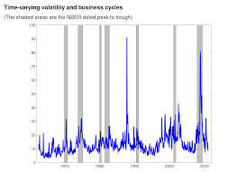
In this chapter we are concerned with variances that change over time, i.e., time-varying variance processes. The model we focus on is called the AutoRegressive Conditional Heteroskedastic (ARCH) model.

This is an example of an ARCH(l) model since the time varying variance h_t is a function of a constant term (a₀) plus a term lagged once, the square of the error in the previous period ( cqe,².,). The coefficients, a₀ and a,, have to be positive to ensure a positive variance. The coefficient a, must be less than 1, otherwise h_t will continue to increase over time, eventually exploding.

Conditional normality means that the distribution is a function of known information at time t -1i.e., when t = 2, (e₂ | I₁,) ~ N(0,a₀ + a₁e₁²) and so on.

The EViews workfile byd.wfl contains the returns to BrightenYourDayLighting. To plot the times series, double-click the variable and select View/ Open Graph/ Line & symbol and click OK.

To generate the histogram, select View/ Descriptive Statistics & Tests/ Histogram and Stats.

Clicking this option gives the distribution below.

2. TESTING FOR ARCH EFFECTS

To test For first order ARCH, regress the squared regression residuals e² on their lags e²_t-1:

where v, is a random term. The null and alternative hypotheses are:

If there are no ARCH effects, then y₁ = 0 and the fit of the testing equation will be poor with a low R². If there are ARCH effects, we expect the magnitude of e² to depend on its lagged values and the R² will be relatively high. Hence, we can test For ARCH effects by checking the significance of y₁, as well as applying the LMtest based on R².

The regression residuals are obtained from the mean equation. The regression of returns on a constant term is shown below.

To generate the regression residuals, select View, select Residual Tests/Heteroskedasticity Tests from the drop down menus.

Then select the ARCH option. Inserting 1 in the Number of lags box means that we are testing for ARCH( 1) effects.

Clicking on OK gives the ARCH test results below.

Since the CM statistic (62.159) is significant, we reject the null hypothesis that there is no first- order ARCH effects. Note that the LM statistic in EViews is calculated as LM = TxR² = 499×0.124568=62.16. Furthermore, the F- and t-statistics (62.16 = 8.4095²) corroborate the presence of first order ARCH effects.

3. ESTIMATING AN ARCH MODEL

To estimate an ARCH model, click Quick/ Estimate equation and select the ARCH option from the drop-down menu in Method.

A screen with an upper Mean equation and a lower Variance and distribution specification section will open up. In the mean equation section, enter the regression of the returns, R, on a constant, C. In the variance and distribution specification section, to estimate an ARCH model of order 1, type a 1 against ARCH.

To obtain the standard errors reported in the text, click on Options (top left hand comer) and then pick the options noted below. As discussed in the text, time series models require an initial starting value, in this case the initial variance h.. The options suggested here set the initial variance to the unconditional sample variance.

Clicking on OK will give the EViews output below. Note that we have used the default Marquardt algorithm to generate these results.

The top section is the mean equation. It shows that the average return is 1.063939. The lower section is the variance equation that gives the result of the ARCH model, namely, that the time varying volatility h_t includes a constant component (0.642140) plus a component which depends on past errors. The shaded line highlights the significant ARCH effects.

To generate the conditional variance series shown in the text, click on Proc and select Make GARCH Variance Series from the drop-down menu.

Clicking opens the window below. We have used H to label the conditional variance.

Clicking on OK creates the series which you can then graph by selecting View / Graph/ Line & Symbol/.

4. GENERALIZED ARCH

To estimate a GARCH(1,1) model, select the option shown below.

Clicking on OK produces the EViews results below.

Recall that the generalized GARCH(1,1) model is of the form:

We also note that we need a₁ + β₁ < 1 for stationarity; if a₁ + β₁ > 1 we have a so-called “integrated GARCH” process, or IGARCH.

The shaded line in the EViews output shows the significance of the GARCH term. These results show that the volatility coefficients, the one in front of the ARCH effect (0.491027) and the one in front of the GARCH effect (0.238007) are both positive and their sum is between zero and one, as required by theory.

5. ASYMMETRIC GARCH

The threshold ARCH model, or T-ARCH, is one example where positive and negative news are treated asymmetrically. In the T-GARCH version of the model, the specification of the conditional variance is:

where y is known as the asymmetry or leverage term.

When y = 0, the model collapses to the standard GARCH form. Otherwise, when the shock is positive (i.e. good news) the effect on volatility is a, but when the news is negative (i.e. bad news) the effect on volatility is a, + y . Hence, so long as y is significant and positive, negative shocks have a larger effect on h_t than positive shocks.

To estimate a threshold GARCH model, select the option shown below.

Clicking OK gives the EViews ouput

Since the coefficient on the asymmetric term (0.492) is significant, we infer that there is evidence that positive and negative shocks have different effects. In particular, when the shock is positive, the estimate of the time-varying volatility is

and when the shock is negative, the estimate of the time-varying volatility is

6. GARCH-IN-MEAN

The equations of a GARCH-in-mean model are shown below:

The first equation is the mean equation; it now shows the effect of the conditional variance on the dependent variable. In particular, note that the model postulates that the conditional variance h_t affects y_t by a factor 0. The other two equations are as before.

To estimate a GARCH in mean model, select the option shown below.

Clicking on OK produces the EViews ouput below.

Since the coefficient on the GARCH in mean term (0.196) is significant, we infer that there evidence that volatility affects returns.

Source: Griffiths William E., Hill R. Carter, Lim Mark Andrew (2008), Using EViews for Principles of Econometrics, John Wiley & Sons; 3rd Edition.

1. GRUNFELD DATA: TWO EQUATIONS

Panel data are data with two dimensions, a time dimension and a cross-section dimension. They typically comprise observations on a number of economic units, such as individuals or firms, over a number of time periods. The use of panel data involves new models, new econometric techniques and new ways of handling the data. EViews has the capacity to estimate a vast array of models, using many different estimation techniques. Also, the user has various options for handling the data and proceeding to estimation. Some but not all of those options will be introduced as we lead you through the examples in Chapter 15 of the text. The first example involves T = 20 time series observations on just N = 2 cross sectional units, the firms General Electric and Westinghouse. The data can be found in the file grunfeld2.dat. We are interested in estimating the two equations

where INV denotes investment, V denotes market value of stock and K denotes capital stock, with the subscripts GE and WE referring to General Electric and Westinghouse, respectively. There are various ways of estimating these two equations depending on what further assumptions are made about the coefficients and the error terms in each of the equations. We first consider separate least squares estimation of each equation.

1.1. Separate least squares estimation

In the following screenshot the two separate equation specifications for the GE and WE equations have been superimposed on the workfile. There is nothing new in these specifications. They are straightforward least squares estimations. With respect to the structure of the workfile, there are two things worth noting. First, the observations are dated with the range and sample specified as annual data from 1935 to 1954. Second, each of the variables has a “subscript”, GE or _WE to signify whether the observations are for General Electric or Westinghouse. These “subscripts” are known as cross section identifiers. They will be important in subsequent sections of this chapter.

The outputs from each of these regressions follow. Note that they confirm the results in Table 15.1 on page 386 of the text.

1.2. Stacking the data

In the previous section we estimated two regression equations with 20 observations for each. As noted in equation (15.6) of the text, the same least squares estimates can be obtained by pooling the observations into one sample of 40, and including intercept and slope dummy variables for each of the coefficients. The standard errors turn out differently, however. With separate least squares estimation we get separate estimates for a²_CE and a²_WE . When the observations are pooled into one sample, the implicit assumption is that a²_GE = a²_VE and only one error variance estimate is obtained.

To obtain the pooled dummy variable estimates, it is convenient to stack the observations into one sample of size 40. In addition to stacking INV, V and K, we will create the required dummy variable by defining DUM WE = 1 and DUM_GE = 0, and also stacking these two series.

series dum we = 1

series dum_ge = 0

We have chosen the notation DUM rather than D as used by the text because EViews reserves D to be used as a difference operator, as was described in Chapter 12. Stacking is carried out by creating a second page in our workfile and storing the stacked series in that page. But, first we name the first page that contains the unstacked data. Go to fProcl, and select Rename Current Page. In the resulting dialog box, call the page unstacked.

To create a new page with the stacked data, go to Proc/Reshape Current Page/Stack in New Page.

A Workflle Stack dialog box appears. The cross section identifiers _GE and _WE are inserted in the Stacking Identifiers box. In the box that says Series to stack into new workflle page, each of the series names is entered without the subscripts (identifiers), and with each identifier replaced by a question mark ?. Leaving the box below that blank will mean that the new series of length 40, with both the GE and WE observations, will be called INV, V, K and DUM.

Notice the second tab in the Workfile Stack box called Page Destination. Click on that. We are keeping the current workfile and naming the new page stacked.

The new workfile page called stacked is illustrated below. Check out the following.

1. The Range is given as 1935 1954 x 2 implying we have two cross sections for the specified time period.
2. The names of the new series that include all 40 observations are INV, V, K and
3. There are two new series ID01 and The first one indicates which observations are GE and which are WE. The second contains the date of each observation.

Open the various series and familiarize yourself with how EViews has set them up.

1.3. Least squares estimation with dummy variables

We are now in a position to obtain the estimates given in Table 15.2 on page 387 of the text. Follow the familiar routine of going to Object/New Object/Equation, name the equation object and fill in the Equation specification.

The variables specified are those that appear in equation (15.6) and Table 15.2 of the text. Notice that we are able to enter the products dum*v and dum*k without creating new series. EViews figures it out and gives you the results.

Something new that has suddenly turned up is another tab called Panel Options. Because you went through a stacking procedure, EViews knows that the data are panel data. Accordingly, it set up a panel workfile structure that specifies a panel range and includes objects describing the cross section and time series components. The panel workfile structure includes Panel Options in the Equation Estimation window. For the moment we do not need these options, but we do consider some of them shortly. Clicking OK reveals the results in Table 15.2 on page 387.

1.4. Introducing the pool object

The dummy variable model estimated in the previous section is given by

Using the substitutions

the dummy variable model can be written as

Estimating this equation will give exactly the same results as those from the earlier dummy variable model in the sense that estimates and standard errors of corresponding coefficients will be equal. We can estimate it from the stacked page of grunfeld2.wfl, using the equation specification

inv (1-dum) dum (1-dum)*v dum*v (1-dum)*k dum*k

Try it! See what you get. Can you match corresponding coefficients with Table 15.2?

We can also get these estimates using a pool object in the unstacked page. Return to the unstacked page and select Object/New Object/Pool. We named the pool object LS_EQNS.

EViews will then ask you for the cross section identifiers which in this case are GE and WE. For this procedure to work, series names should be expressed with a common component such as INV, K and V and with a cross section identifying component like _GE and WE.

Then click on Estimate. Wow! Look at all the boxes you have to fill in. Don’t be scared. At the moment we are only concerned with two of them.

1. For the Dependent variable we have written INV?. Writing it this way, with the question mark, tells EViews to consider all values on investment. Remember that you have already told EViews about the cross-section identifiers. It won’t forget.
2. The other box that is filled in is the Cross-section specific coefficients We chose this one because we want to allow the General Electric coefficients to be different from the Westinghouse coefficients. If you wanted them to be the same, you would choose the Common coefficients box. If you wanted the coefficients for some variables to be the same and some to be different, you can write some of the explanatory variable names in one box and some in the other.
3. Because we are estimating the equation by straightforward least squares, we do not need to change the default settings in the Estimation method

The results follow. They are equivalent to those in Table 15.2, although at first glance you might not think so. We can see the equivalence by noting that

1.5. Seemingly unrelated regressions

The coefficient estimates obtained in the previous section were obtained under the assumption that σ_GE = σ²_WE, and that the errors for the Westinghouse and General Electric equations, in the same year, are uncorrelated, cov(e_GE, e_WE) = 0. Seemingly unrelated regression estimates are obtained under the assumptions σ²_GE # σ²_WE and cov(e_GE ,e_WE,) # 0 . To obtain them we proceed exactly as we did in the previous section, with one slight modification. Can you remember the steps? Set up a pool object. Give it a name. This time we will call it SUR. Fill in the cross-section identifiers. Click Estimate. Fill in the Dependent variable and Cross-section specific coefficients boxes as before. The new thing that you need to do this time is to select Cross­section SUR from the drop-down Weights menu in the Estimation method box.

The results appear below. Compare them with Table 15.3 on page 388 of the text. The following points are worth noting.

1. In the output the coefficients are ordered according to variable. In Table 15.3 they are ordered according to equation.
2. EViews calls the estimation method Pooled EGLS (estimated generalized least squares). The SUR estimator is a particular kind of generalized least squares estimator.
3. Although the coefficient estimates are identical to those in Table 15.3, the standard errors are not. The difference arises because EViews uses T as the divisor when estimating the error variances and covariance, whereas the degrees of freedom corrected divisor T -K was used for the results in Table 15.3. Both are popular. To reconcile the two, consider the last standard error reported from both places and note that

1.6. Testing contemporaneous correlation

In the context of the two-equation SUR model, a test for contemporaneous correlation is a test of H₀: cov(e_GE,e_WE ) = 0. The relevant test statistic, described on page 389 of the text, is LM = T x r²_GE.WE where r²_GE.WE is the squared correlation between the least squares residuals from the two equations. To get this correlation return to the pool object LS EQNS (we want least squares residuals not SUR residuals), open it, and select View/Residuals/Correlation Matrix.

From the resulting matrix, we have r²_GE.WE = (0.728965)² = 0.53139 , giving a test statistic value of LM = 20×0.53139 = 10.628. The command

scalar pval = 1 – @cchisq(10.6278,1)

yields a p-value of 0.0011. We reject H₀ and conclude that contemporaneous correlation between the equation errors exists.

1.7. Testing cross-equation restrictions

So far we have been assuming that General Electric and Westinghouse have different coefficients. Could they be the same? To answer this question we test the hypothesis

This hypothesis can be tested using the Wald test option from SUR estimation. For carrying out the test we can follow the same steps as described in Chapter 6, although in this case the formulas for the test statistics are more complicated than we have divulged. Also, special care must be exercised to make sure we are testing the coefficients that we want to test. Return to the SUR output. Note the order of the coefficients. This is the order in which EViews stores them in the C vector. Consequently, writing the null hypothesis in terms of EViews coefficients, we have

H₀: C(1)=C(2), C(3)=C(4), C(5)=C(6)

Select View/Coefficient TestsAVald – Coefficient Restrictions. Enter the following restrictions in the Wald test box.

In the lower part of the output, the normalized restrictions are P_1.GE – P_1.WE = 0, P_2.GE – P_2.WE = 0  and P_{3 G£} -P₃._TO =0. Estimates of the left hand sides of the restrictions and their standard errors appear in the columns Value and Std. Err. The F- and y²-values for the test are given in the upper part of the output, along with their corresponding ^-values. The hypothesis of equal coefficients is rejected.

There is a discrepancy between the values in the text on pages 390-1 and those in the above output. Those in the text are F = 2.92 and x² = 8.77. The difference is again attributable to the treatment of a degrees of freedom correction when estimating the error variances and covariance. To convert the EViews values to the text values, we multiply by (17/20).

2. GRUNFELD DATA: TEN FIRMS

A more complete set of the Grunfeld data comprising T = 20 observations on A = 10 firms can be found in the workft\e grunfeld.wfl. The contents of this workfile are displayed below.

This file contains the familiar series INV, V and K and two new series I and T. The series I identifies observations for the i-th firm, i = 1,2,…, 10 . The series T identifies observations for the t-th time period, t = 1,2,…,20. The Range and Sample are both simply set at 1 200 without recognition of the panel structure of the data. So that EViews is fully informed, we begin this section by specifying the panel structure.

2.1. Structuring the workfile

Go to Proc/Structure/Resize Current Page. A Workfile structure dialog box appears. There are various options that we could choose from the drop-down menu Workfile structure type. Since we have the identifying series / and T in the workfile, we choose undated with ID series and insert the names of these series in the Identifier series box.

When you return to the workfile, you will see extra information under Range that says Dim(10,20). In other words, the panel dimension is (10×20). EViews has figured out this dimension by checking the values in I and T.

2.2. Fixed effects using dummy variables

Table 15.4 on page 392 of the text presents estimates of the investment functions for the 10 firms assuming (1) all firms have the same coefficients on V and K, (2) each firm has a different intercept, (3) the error variances are the same for all firms, and (4) there is no contemporaneous correlation between errors of different firms. Taken together, these assumptions comprise those of a standard fixed effects model. The different intercept terms are known as fixed effects. The fixed effects model can be estimated in one of two ways. Dummy variables can be included for each of the firms and the constant omitted. In this case the coefficients of the dummy variables are the intercepts (fixed effects). Alternatively, the data can be expressed in terms of deviations from firm means and estimated without any intercepts, as described on page 394 of the text. We will first estimate the model by including dummy variables. Later we consider EViews automatic fixed effects option, and relate it back to our results for the dummy variable specification. We do not explicitly consider estimation using data expressed as deviations from firm means, although that is undoubtedly the approach taken by EViews automatic command.

We generate the dummy variable series by using a sequence of logical generate commands. For example, the command

series d1 = (i=1)

generates a series D1 that is equal to one when (i=1) is true and equal to zero when (i=1) is false. Ten such commands are needed, one for each dummy variable.

To estimate the model, proceed to the Equation specification in the usual way. Enter the dependent variable INV, followed by each of the dummy variables, V and K. You will have noticed the Panel options tab at the top of the Equation estimation window. It is not needed. You might be tempted to select fixed effects. That would be wrong. Including the dummy variables means the fixed effects are already included. If you try to do it twice, EViews will get upset and send you a nasty singular matrix message.

Compare the above output with that in Table 15.4 of the text. Note the way EViews describes the panel structure in the top portion of the output.

2.3. Testing the effects

A test likely to be of interest is one that checks whether the intercepts for all Firms could be identical. If they are, one can use a pooled least squares regression estimated from the 200 observations without any regard for the panel structure. Open the Wald test box by going to View/Coefficient Tests/Wald – Coefficient Restrictions. We want to test whether the 10 intercept coefficients are equal. Another way of putting it is we want to replace 10 coefficients with one coefficient. To do so involves 9 restrictions. There are a number of different ways of writing these restrictions. One way appears in the box below. Note that the intercepts represent the first 10 coefficients and so they will be numbered C(l), C(2), …, C(10). Another alternative is to set C(l) = C(2), C(l) = C(3), …, C(l) = C(10). You will be able to think of other ways.

The upper panel of the test outcome appears below. Notice that the F-value is the same as that on page 393 of the text, obtained using restricted and unrestricted sums of squared errors. The relationship between the two test values is x² =9xF , with 9 being the degrees of freedom for the x² -test and the numerator degrees of freedom for the F-test. With p-values of 0.0000, both tests clearly reject the null hypothesis of equal intercepts.

2.4. Pooled least squares

The pooled least squares estimates that make no special assumptions to accommodate the panel structure are given in Table 15.7 on page 395 of the text. No special commands are required to produce these estimates. Following the usual steps, leads to the Equation specification and results that appear below.

2.5. The fixed effects estimator

Now consider EViews automatic command for estimating a Fixed effects (dummy variable) model. You Fill in the same Equation specification as you did for the pooled least squares estimator in the previous section, but this time you need to click on the Panel options tab and choose Fixed for the Cross-section Effects specification.

The upper part of the output appears below. You should notice that the estimates for the coefficients of V and K are identical to those obtained when we explicitly included the dummy variables in Section 15.2.2. Also, if you took time to do the arithmetic, you would discover that the new intercept -58.729 is equal to the average of the dummy variable coefficients obtained earlier.

a. Retrieving the fixed effects

Sometimes the fixed effects (intercept estimates) are of special interest. They can be used to analyze the extent of firm heterogeneity and to examine any particular firms that may be of interest. For many examples the number of fixed effects is enormous and so rather than print them on the output, Eviews puts them in a special spreadsheet. To locate this spreadsheet go to View/Fixed/Random Effects/Cross-section Effects.

The spreadsheet for the fixed effects for each of the 10 firms is given in the left-hand side of the panel below. A comparison with the dummy variable coefficients from Table 15.4 reveals that they are not the same. The difference is that EViews has expressed them in terms of deviations form the mean of -58.729 that was reported on the output. To get the original fixed effects you add the mean as is done on the right-hand side of the below panel.

b. Testing the fixed effects

Can we use the fixed effects output to test for equality of the fixed effects (dummy variable coefficients) like we did earlier using the dummy variable specification? The answer is yes. Go to View/Fixed/Random Effects Testing/Redundant Fixed Effects – Likelihood Ratio.

Two versions of the likelihood ratio test appear in the output, an E-test and a x² -test. The E-test is identical to the one we considered earlier, and gives the same test results. The x²-test has a different origin, and so leads to a different test value. The details are beyond the level of our current description, but you can get a feel for where it comes from by checking equation (C.25) on page 537 of the text.

3. THE NLS PANEL DATA

The data in the file nls_panel.wfl is from the National Longitudinal Surveys conducted by the U.S. Department of Labor. This file is a large one that, in its current form, cannot be saved by the Student Version of EViews. We can nevertheless use the Student Version to analyze the data. After you have finished estimation, if you wish to save your results, you will need to reduce the range of the workfile structure and delete some of the series until the file is small enough to be saved by EViews Student Version. When saving it, name it differently, say nls results.wfl. You will then have two files, the original one with the data and another one with your results. This is an inconvenient state of affairs, but not an impossible scenario. The other alternative is to pay more for convenience and buy the EViews full version.

Opening the file reveals 3580 observations with a panel structure comprising 5 time series observations (1982, 1983, 1987, 1988) on 716 individuals.

We can check the data against that in Table 15.8 by collecting those variables into a group and examining the following spreadsheet.

3.1. Fixed effects estimation

The first model estimated using the NLS panel is a fixed effects model with In (WAGE) as the dependent variable and explanatory variables EXPER, EXPER2, TENURE, TENURE2, SOUTH and UNION. It is also suggested that we try a fixed effects model with EDUC and BLACK included to see what happens. Estimation should fail because EDUC and BLACK are constant over time for each individual. Their effects will be captured by the individual fixed effects. The Equation specification and Effects specification (selected form the Panel options) for this model are

This is a message that you will see if you try to estimate a model with perfect collinearity among the explanatory variables. In fact, EViews is being kind. The relevant matrix is singular not just “nearly” singular. We have not been specific about the matrix to which EViews refers. At this stage of your career is is sufficient to know that the singularity is caused by collinear explanatory variables.

After dropping the offending variables EDUC and BLACK, the specification is

The output follows. Note the correspondence with the results in Table 15.9 on page 397 of the text.

To test for the presence of individual differences we test the equality of the fixed effects as described in Section 15.2.5b. Go to View/Fixed/Random Effects Testing/Redundant Fixed Effects – Likelihood Ratio.

The resulting test details confirm the F-value of 19.66 reported on page 398 of the text.

3.2. Random effects estimation

Individual effects that were modeled by fixed coefficients in the fixed effects model are treated as random draws from a larger population in the random effects model. For estimation purposes they become part of the error term. Also, estimation of the random effects model takes into account variation between individuals as well as variation within individuals. For our data set, this means it is possible to include EDUC and BLACK in the model. Doing so leads to the following Equation and effects specifications.

The output that follows yields the results in Table 15.10 on page 402 of the text. In the lower part of the output, cross section random refers to the estimate o_a =0.3291 and idiosyncratic random refers to the estimate o_e = 0.1951. The values in the column rho are the proportions of total error variance attributable to each of the components. Thus,

3.3. The Hausman test

The ability of the random effects model to take into account variation between individuals as well as variation within individuals makes it an attractive alternative to fixed effects estimation. However, for the random effects estimator to be unbiased in large samples the effects must be uncorrelated with the explanatory variables, an assumption that is often unrealistic. This assumption can be tested using a Hausman test. The Hausman test is a test of the significance of the difference between the fixed effects estimates and the random effects estimates. Correlation between the random effects and the explanatory variables will cause these estimates to diverge; their difference will be significant. If the difference is not significant, there is no evidence of the offending correlation. The differences between the two sets of estimates can be tested separately using t-tests,, or as a block using a x²-test.

You can ask EViews to perform a Hausman test by opening the random-effects estimated equation and going to View/Fixed/Random Effects Testing/Correlated Random Effects – Hausman Test.

For the wage equation we get the following results. The value of the -statistic for testing differences between all coefficients is x² = 20.437 . Its corresponding p-\alue of 0.0023 suggests the null hypothesis of no correlation between the explanatory variables and the random effects should be rejected. The p-values for separate tests on the differences between each pair of coefficients are given in the column Prob. The results here are mixed. At a 5% significance level, the null hypothesis is rejected for TENURE2, SOUTH and UNION, but not for EXPER, EXPER1 and TENURE. These results are slightly different to those reported on pages 205-206 of the text, but not enough to suggest anything is wrong. Differences may have occurred because of different covariance matrix estimators.

Source: Griffiths William E., Hill R. Carter, Lim Mark Andrew (2008), Using EViews for Principles of Econometrics, John Wiley & Sons; 3rd Edition.

1. MODELS WITH BINARY DEPENDENT VARIABLES

We will illustrate binary choice models using an important problem from transportation economics. How can we explain an individual’s choice between driving (private transportation) and taking the bus (public transportation) when commuting to work, assuming, for simplicity, that these are the only two alternatives? We represent an individual’s choice by the dummy variable

If we collect a random sample of workers who commute to work, then the outcome y will be unknown to us until the sample is drawn. Thus, y is a random variable. If the probability that an individual drives to work is p, then P[y = 1] = p . It follows that the probability that a person uses public transportation is P[y = 0] = 1 – p. The probability function for such a binary random variable is

where p is the probability that;; takes the value 1. This discrete random variable has expected value E(y) = p and variance var( y) = p(1-p).

What factors might affect the probability that an individual chooses one transportation mode over the other? One factor will certainly be how long it takes to get to work one way or the other. Define the explanatory variable

x – (commuting time by bus – commuting time by car)

There are other factors that affect the decision, but let us focus on this single explanatory variable. A priori we expect that as x increases, and commuting time by bus increases relative to commuting time by car, an individual would be more inclined to drive. That is, we expect a positive relationship between x and p, the probability that an individual will drive to work.

1.1. Examine the data

Open the workfile transport.wfl. Save the workfile with an new name to transportchapl6.wfl so that the original workfile will not be changed. Highlight the series AUTOTIME, BUSTIME, DTIME and AUTO in order. Double-click in the blue to open the Group. The data are shown on the next page.

The key point is that AUTO, which is to be the dependent variable in the model, only takes the values 0 and 1.

Obtain the descriptive statistics from the spreadsheet view: Select View/Descriptive Stats/Common Sample.

The summary statistics will be useful later, but for now notice that the SUM of the AUTO series is 10, meaning that of the 21 individuals in the sample, 10 take their automobile to work and 11 take public transportation (the bus.)

1.2. The linear probability model

Our objective is to estimate a model explaining why some choose AUTO and some choose BUS transportation. Because the outcome variable is binary, its expected value is the probability of observing AUTO = 1,

The model

is called the linear probability model. It looks like a regression, but as noted in POE, page 420, there are some problems. Nevertheless, apply least squares using y = A UTO and x = DTIME.

The problems with this estimation procedure can be observed by examining the predicted values, which we call PHAT. In the regression window select the Forecast button

[Forecast]

Fill in the dialog box with a Forecast name.

An object PHAT appears in the workfile. Double-click to open. Examining just a few observations shows the unfortunate outcome that the linear probability model has predicted some probabilities to be greater than 1 or less than 0.

Now, examine the summary statistics for PHAT from the spreadsheet view, by selecting View/Descriptive Statistics & Tests/Stats Table.

Note that the average value of the predicted probability is .476, which is exactly equal to the fraction (10/21) of riders who choose AUTO in the sample. But also note that the minimum and maximum values are outside the feasible range.

1.3. The probit model

The probit statistical model expresses the probability p that v takes the value 1 to be

where Φ(z) is the probit function, which is the standard normal cumulative distribution function (CDF). This is a nonlinear model because the parameters β₁ and β₂ are inside the very nonlinear function Φ(•). Using numerical optimization procedures, that are outside the scope of this book, we can obtain maximum likelihood estimates. From the EViews menubar select Quick/Estimate Equation. In the resulting dialog box, click the pull down list in the Method section of Estimation settings

A long list of options appears. Choose BINARY.

The estimation settings should look like

In the Equation specification box enter the equation as usual, but select the radio button for Probit.

Click OK. The estimation results appear on the next page. In most ways the output looks similar to the regression output we have seen many times. The Coefficients, Std. Error and Prob. columns are familiar. There are many items included in the output you will not understand, and we are just omitting. However, we note the following:

• The Method: ML means that the model was estimated by maximum likelihood.
• The usual t-Statistic has been replaced by z-Statistic. The reason for this change is that the standard errors given are only valid in large samples. As we know the t-distribution converges to the standard normal distribution in large samples, so using “z” rather than “t” recognizes this fact. The p-values Prob. are calculated using the N(0,1) distribution rather than the t-distribution.

• In the bottom portion of the output we see an R² value called McFadden R-squared. This is not a typical R” and cannot be interpreted like an R². As a child your mother pointed to a pan of boiling water on the stove and said Hot! Don’t touch! We have a similar attitude about this value. We don’t want you to “get burned,” so please disregard this number until you know much more.
• The LR statistic is comparable to the overall F-test of model significance in regression. It is a test statistic for the null hypothesis that all the model coefficients are zero except the intercept, against the alternative that at least one of the coefficients is not zero. The LR statistic has a chi-square distribution if the null hypothesis is true, with degrees of freedom equal to the number of explanatory variables, here Prob(LR statistic) is the p-value for this test, and it is used in the standard way. If p < a then we reject the null hypothesis at the a level of significance.

1.4. Predicting probabilities

The “prediction” problem in probit is to predict the choice by an individual. We can predict the probability that individuals in the sample choose AUTO. In order to predict the probability that an individual chooses the alternative AUTO (y) = 1 we can use the probability model p = Φ(β₁ + β₂x) using estimates β₁ = -0.0644 and β₂ = 0.02999 of the unknown parameters obtained in the previous section.. Using these we estimate the probability p to be

By comparing to a threshold value, like 0.5, we can predict choice using the rule

The predicted probabilities are easily obtained in EViews. Within the probit estimation window select Forecast.

In the resulting Forecast dialog box choose the Series to forecast to be the Probability, and assign the Forecast name PHAT PROBIT. Click OK.

Open the series PHAT_PROBIT by double-clicking the series icon in the workfile window. The values of the predicted probabilities are given for each individual in the sample, based on their actual DTI ME.

It is useful to see that these predicted probabilities can be computed directly using the EViews function @cnorm which is the CDF of a standard normal random variable, what we have called “Φ”. EViews places the estimates of the unknown parameters in the coefficient vector C,

The predicted probabilities from the two methods are the same

1.5. Marginal effects in the probit model

In this model we can examine the effect of a one unit change in jc on the probability that y = 1 by considering the derivative, which is often called marginal effect by economists.

This quantity can be computed using the EViews function @dnorm, which gives the standard normal density function value, that we have represented by Φ. To generate the series of marginal effects for each individual in the sample, enter the command

series mfx_probit = @dnorm(c(1)+c(2)*dtime)*c(2)

The marginal effect at a particular point uses the same calculation for a particular value of DTIME, such as 20.

scalar mfx_probit_20 = @dnorm(c(1)+c(2)*20)*c(2)

EViews is very powerful, and one of its features is the calculation of complicated nonlinear expressions involving parameters and computed their standard error by the “Delta” method. In the PROBIT estimation w indow, select View/Coefficient Tests/Wald – Coefficient Restrictions.

In the dialog window enter the expression for the marginal effect, assuming DTIME = 20, setting it equal to zero as if it were a hypothesis test.

This returns the F-test statistic for the null hypothesis that the marginal effect is zero. Thep-value is 0.005 leading us to reject the null hypothesis that additional BUS time has no effect on the probability of AUTO travel when DTIME = 20. Furthermore, the Value and the Std. Err. are computed. The value matches the scalar MFX PROBIT 20 computed earlier, and we now have a standard error that can be used to construct a confidence interval. Very cool.

To make the estimations using the Logit model simply change the Equation Estimation entries to

2. ORDERED CHOICE MODELS

In POE Chapter 16.3 we considered the problem of choosing what type of college to attend after graduating from high school as an illustration of a choice among unordered alternatives. However, in this particular case there may in fact be natural ordering. We might rank the possibilities as

The usual linear regression model is not appropriate for such data, because in regression we would treat the y values as having some numerical meaning when they do not. When faced with a ranking problem, we develop a “sentiment” about how we feel concerning the alternative choices, and the higher the sentiment the more likely a higher ranked alternative will be chosen. This sentiment is, of course, unobservable to the econometrician. Unobservable variables that enter decisions are called latent variables, and we will denote our sentiment towards the ranked alternatives by y*, with the “star” reminding us that this variable is unobserved.

As a concrete example, let us think about what factors might lead a high school graduate to choose among the alternatives “no college,” “2-year college” and “4-year college” as described by the ordered choices above. For simplicity, let us focus on the single explanatory variable GRADES. The model is then

This model is not a regression model because the dependent variable is unobservable. Consequently it is sometimes called an index model.

Because there are M = 3 alternatives there are M -1 = 2 thresholds μ₁ and μ₂, with μ₁ < μ₂. The index model does not contain an intercept because it would be exactly collinear with the threshold variables. If sentiment towards higher education is in the lowest category, then y* < μ₁ and the alternative “no college” is chosen, if μ₁ < y* < μ₂ then the alternative “2-year college” is chosen, and if sentiment towards higher education is in the highest category, then y* > μ₂ and “4- year college” is chosen. That is,

We are able to represent the probabilities of these outcomes if we assume a particular probability distribution for y , or equivalently for the random error e_i. If we assume that the errors have the standard normal distribution, N(0,1), and the CDF is denoted d>. an assumption that defines the ordered probit model, then we can calculate the following:

and the probability that y = 3 is

In this model we wish to estimate the parameter p, and the two threshold values pi and p2. These parameters are estimated by maximum likelihood.

In EViews open the workfile nelssmalLwfl. Save it under the name nels small oprobitwfl. The dependent variable of interest is PSECHOICE and the explanatory variable is GRADES. Select Quick/Estimate Equation. In the drop down menu of estimation methods choose Ordered Choice.

Enter the estimation equation with NO INTERCEPT. Make sure the Normal radio button is selected so that the model is Ordered Probit.

The results, edited to remove things that are not of interest, are

The coefficient of GRADES is the maximum likelihood estimate (3. The values labeled LIMIT_2:C(2) and LIMIT 3:C(3) are the maximum likelihood estimates of p, and p₂. The notation points out that the these parameter estimates are saved into the coefficient vector as C(2) and C(3). C(l) contains J3. Name this equation OPROBIT.

2.1. Ordered probit predictions

To predict the probabilities of various outcomes, as shown on page 436 of POE, we can again use the computing abilities of EViews. In the OPROBIT estimation window select View/Coefficient Tests/Wald – Coefficient Restrictions.

To compute the probability that a student with GRADES = 2.5 will attend a 2-year college we calculate

Enter into the Wald Test dialog box

The predicted probability is the relatively low 0.078, which makes sense because GRADES =2.5 is very high on the 13 points scale..

We can use the same general approach to compute the probabilities for each option for all the individuals in the sample. Recall that the maximum likelihood estimates of μ₁ and μ₂ are saved into the coefficient vector as C(2) and C(3). C(1) contains β.

Open a Group showing the GRADES, PSECHOICE and the predicted probabilities.

A standard procedure is to predict the actual choice using the highest probability. Thus we would predict that person 1 would attend no college, and the same with person 2. Both of these predictions are in fact incorrect because they choose a 2-year college. Individual 3 we predict will attend a 4-year college, and they did.

In the EViews window containing the estimated model OPROBIT, select View/Dependent Variable Frequencies

We see the choices made in the data

Now select View/Prediction Evaluation.

Using the “highest probability” prediction rule, EViews calculates

This model, being a very simple one, has a difficult time predicting who will attend 2-year colleges, being incorrect 100% of the time.

2.2. Ordered probit marginal effects

The marginal effects in the ordered probit model measure the changed in probability of choosing a particular category given a 1-unit change in an explanatory variable. The calculations are different by category. The calculations involve the standard normal probability density function, denoted Φ and calculated in EViews by @dnorm. For example the marginal effect of GRADES on the probability that a student attends no college is

In the OPROBIT window select View/Coefficient Tests/Wald – Coefficient Restrictions. In the dialog box enter

Recalling that a higher value of GRADES is a poorer academic performance, we see that the probability of attending no college increases by 0.045 for a student with GRADES = 5.

The marginal effect calculation can be carried out for each person in the sample using the command

series mfx_y1 = – @dnorm(c(2) – c(1)*grades)*c(1)

Open a Group showing GRADES and this marginal effect. Note that increasing GRADES by 1- point (worse grades) increases the probabilities of attending no college, but for students with better grades (GRADES lower) the effect is smaller.

3. MODELS FOR COUNT DATA

If Y is a Poisson random variable, then its probability function is

The factorial (!) term y! = y x (y-1)x(y-2) x…x 1. This probability function has one parameter, λ, which is the mean (and variance) of Y. In a regression model we try to explain the behavior of E(y) as a function of some explanatory variables. We do the same here, keeping the value of E(y)>0 by defining

This choice defines the Poisson regression model for count data.

Prediction of the conditional mean of y is straightforward. Given the maximum likelihood estimates β₁ and β₂, and given a value of the explanatory variable x₀, then

This value is an estimate of the expected number of occurrences observed, if x takes the value x₀. The probability of a particular number of occurrences can be estimated by inserting the estimated conditional mean into the probability function, as

The marginal effect of a change in a continuous variable x in the Poisson regression model is not simply given by the parameter, because the conditional mean model is a nonlinear function of the parameters. Using our specification that the conditional mean is given by

and using rules for derivatives of exponential functions, we obtain the marginal effect

To estimate this marginal effect, replace the parameters by their maximum likelihood estimates, and select a value forx. The marginal effect is different depending on the value ofx chosen.

To illustrate open the workfile olympics.wfl. You will find a very rude message.

This workfile is too large because there are too many observations. The definition file Olympics.def shows that there are 1610 observations.

We can still operate with the workfile, but we cannot save it even if we delete some variables. Give this a try, deleting the variables that are needed in this example.

The example in the book uses only data from 1988. To modify the sample, click the Sample button on the EViews main menu.

In the Sample dialog box add the IF condition

The workfile window now shows that the estimation sample is 179 observations from the year 1988.

Despite these changes the file still cannot be saved with the Student Version of EViews 6. Your options are to switch to the full version, or to make sure you print out all intermediate results as you go along.

3.1. Examine the data

Open a group consisting of MEDALTOT, POP and GDP. Obtain summary statistics for the individual samples

Finding the summary statistics for individual samples is important when some observations are missing, or NA.

Note that there are 152 observations for MEDALTOT, 176 for POP and 179 for GDP.

Obtaining summary statistics for the Common Sample we find that 151 observations are available on all 3 variables.

3.2. Estimating a Poisson model

To estimate the model by maximum likelihood choose Quick/Estimate Equation. In the dialog box make the choices shown below.

The estimated model is

Note that the number of observations used in the estimation is only 151, which is the number of observations common to all variables.

Despite the fact that the workfile cannot be saved, we save these estimation results as an object named POISSON REG.

3.3. Prediciting with a Poisson model

In the estimation window click Forecast. Choose the Series to forecast as Expected dependent var. and assign a name

Recall that the expected value of the dependent variable, in a simple model, is given by

The forecast can be replicated using the following command

We have shown a few values.

To compute the predicted mean for specific values of the explanatory variables we again use the trick of applying the “Wald test.” Select View/Coefficient TestsAVald – Coefficient Restrictions. We must choose some values for POP and GDP at which to evaluate the prediction. Enter the median values from the individual samples for POP and GDP.

The result shows that for these population and GDP values we predict that 0.8634 medals will be won.

3.4. Poisson model marginal effects

As shown in POE equation (16.29) the marginal effects in the simple shown in the simple Poisson model

This marginal effect is correct if the values of the explanatory variable x is not transformed. In the Olympics medal example the explanatory variables are in logarithms, so the model is

and the marginal effect is, using the chain rule of differentiation,

While this does not necessarily look very pretty, it has a rather nice interpretation. Rearrange it as

Are you still not finding this attractive? This quantity can be called a semi-elasticity, because it expresses the change in E(y) given a 1% change in x. Recalling that E(y_i ) = λ_i we can make one further enhancement that will leave you speechless with joy. Divide both sides by E(y) to obtain

The parameter β₂ is the elasticity of the output y with respect to x. A 1 % change in x is estimated to change E[y) by β₂%.

In the Olympics example, based on the estimation results, we conclude that a 1% increase population increases the expected medal count by 0.18%, and a 1% in GDP increases expected medal count by 0.5766%.

4. LIMITED DEPENDENT VARIABLES

The idea of censored data is well illustrated by the Mroz data on labor force participation of married women. Open the workfile mroZ’Wfl. You will receive an unpleasant warning when using the Student Version of EViews 6:

However, this problem can be fixed by deleting some variables. Delete the variables indicated below.

EViews now tells us we are OK, can save the workfile

Save the workfile as mrozjtobitwfl to as to keep the original file intact.

A Histogram of the variable HOURS shows the problem with the full sample. There are 753 observations on the wages of married women but 325 of these women did not engage in market work, and thus their HOURS = 0, leaving 428 observations with positive HOURS.

4.1. Least squares estimation

We are interested in the equation

The question is “How shall we treat the observations with HOURS = 0”?

A first solution is to apply least squares to all the observations. Select Quick/Estimate Equation and fill in the Equation Estimation dialog box as follows:

The estimation results are

Repeat the estimation using only those women who “participated in the labor force.” Those women who worked are indicated by a dummy variable LFP which is 1 for working women, but zero otherwise.

The estimation results are shown below. Note that the included observations are 428. The estimation results now show the effect of education (EDUC) to have a negative, but insignificant, affect on HOURS. In the estimation using all the observations EDUC had a positive and significant effect on HOURS.

The least squares estimator is biased and inconsistent for models using censored data.

4.2. Tobit estimation and interpretation

An appropriate estimation procedure is Tobit, which uses maximum likelihood principles. Select Quick/Estimate Equation. In the Equation Estimation window fill in the options as shown below. Tobit estimation is predicated upon the regression errors being Normal, so tick that radio button. In our cases the observations that are “censored” take the actual value 0, and the dependent variable is said to be Left censored because 0 is a minimum value and all relevant values of HOURS are positive. The Estimation settings show the method to include Tobit.

The estimation output shows the usual Coefficient and Std. Error columns. Instead of a t- Statistic EViews reports a z-Statistic because the standard errors are only valid in large samples, making the test statistic only valid in large samples, and in large samples a t-statistic converges to the standard normal distribution. The p-value Prob. is based on the standard normal distribution.

The parameter called SCALE:C(6) is the estimate of σ, the square root of the error variance. This value is an important ingredient in Tobit model interpretation. As noted in POE, equation (16.35), the marginal effect of an explanatory variable in a simple model, is

where as usual Φ is the CDF of a standard normal variable. To evaluate the marginal effect of EDUC on HOURS, given that HOURS > 0, we can use Wald test dialog box. Select View/Coefficient Tests/Wald – Coefficient Restrictions. Enter in the expression for the marginal effect of EDUC at the sample means, as shown on page 447 of POE.

The obtained value is slightly different than the value in the text. Slight differences in results are inevitable when carrying out complicated nonlinear estimations and calculations. The maximum likelihood routines are all slightly different, and stop when “convergence” is achieved. These stopping rules are different from one software package to another.

4.3. The Heckit selection bias model

If you consult an econometrician concerning an estimation problem, the first question you will usually hear is, “How were the data obtained?” If the data are obtained by random sampling, then classic regression methods, such as least squares, work well. However, if the data are obtained by a sampling procedure that is not random, then standard procedures do not work well. Economists regularly face such data problems. A famous illustration comes from labor economics. If we wish to study the determinants of the wages of married women we face a sample selection problem. If we collect data on married women, and ask them what wage rate they earn, many will respond that the question is not relevant since they are homemakers. We only observe data on market wages when the woman chooses to enter the workforce. One strategy is to ignore the women who are homemakers, omit them from the sample, then use least squares to estimate a wage equation for those who work. This strategy fails, the reason for the failure being that our sample is not a random sample. The data we observe are “selected” by a systematic process for which we do not account.

A solution to this problem is a technique called Heckit, named after its developer, Nobel Prize winning econometrician James Heckman. This simple procedure uses two estimation steps. In the context of the problem of estimating the wage equation for married women, a probit model is first estimated explaining why a woman is in the labor force or not. In the second stage, a least squares regression is estimated relating the wage of a working woman to education, experience, etc., and a variable called the “Inverse Mills Ratio,” or IMR. The IMR is created from the first step probit estimation, and accounts for the fact that the observed sample of working women is not random.

The econometric model describing the situation is composed of two equations. The first, is the selection equation that determines whether the variable of interest is observed. The sample consists of N observations, however the variable of interest is observed only for n < N of these. The selection equation is expressed in terms of a latent variable z* which depends on one or more explanatory variables w,., and is given by

For simplicity we will include only one explanatory variable in the selection equation. The latent variable is not observed, but we do observe the binary variable

The second equation is the linear model of interest. It is

A selectivity problem arises when y_t is observed only when Z; = 1, and if the errors of the two equations are correlated. In such a situation the usual least squares estimators of J3, and (3₂ are biased and inconsistent.

Consistent estimators are based on the conditional regression function

where the additional variable λ_i is “Inverse Mills Ratio.” It is equal to

where, as usual, Φ(.) denotes the standard normal probability density function, and Φ(.) denotes the cumulative distribution function for a standard normal random variable. While the value of a is not known, the parameters y₁ and y₂ can be estimated using a probit model, based on the observed binary outcome z_i Then the estimated IMR,

First, let us estimate a simple wage equation, explaining \n{WAGE) as a function of the woman’s education, EDUC, and years of market work experience (EXPER), using the 428 women who have positive wages. Select Quick/Estimate Equation. Fill the dialog box as

Heckit estimation begins with a probit model estimation of the “participation equation,” in which LFP is taken to be a function of AGE, EDUC, a dummy variable for whether or not the woman as children (KIDS) and her marginal tax rate MTR. Create the dummy variable KIDS using

series kids = (kidsl6 + kids618 > 0)

Select Quick/Estimate equation and fill in the dialog box as shown.

Using all the sample data we obtain

In the Forecast dialog box choose the radio button for Index and give this variable a name.

The inverse Mills ratio is then calculated using the EViews functions for the standard normal pdf @dnorm and the standard normal CDF @cnorm.

series imr = @dnorm(lfpf)/@cnorm(lfpf)

Include the IMR into the wage equation as an explanatory variable, using only those women who were in the labor force and had positive wages.

This two-step estimation process is a consistent estimator, however the standard errors Std. Error do not account for the fact the IMR is in fact estimated. If the errors are homoskedastic, we however can carry out a test of the significance of the IMR variable based on the /-statistic that is reported by EViews. This is because under the null hypothesis that there is no selection bias the coefficient of IMR is zero, and thus under the null hypothesis the usual t-test is valid. Here we reject the null hypothesis of no selection bias and conclude that using the two-step Heckit estimation process is needed.

The resulting t-statistic is still significant at the .05 level.

Correct standard errors for the two step estimation procedure are difficult to obtain without specially designed software. Such options, and maximum likelihood estimation of the Heckit model, are available in Limdep and Stata software packages.

Source: Griffiths William E., Hill R. Carter, Lim Mark Andrew (2008), Using EViews for Principles of Econometrics, John Wiley & Sons; 3rd Edition.

1. OBTAINING DATA FROM THE INTERNET

Up to now we have taken you through various econometric methodologies and applications using already prepared EViews workfiles. In this chapter, we show you how to create a workfile and how to import data from an Excel spreadsheet. The first step is to create the Excel data file.

Getting data for economic research is much easier today than it was years ago. Before the Internet, hours would be spent in libraries, looking for and copying data by hand. Now we have access to rich data sources which are a few clicks away.

Suppose you are interested in analyzing the GDP of the United States. As suggested in Chapter 17, the website Resources for Economists contains a wide variety of data, and in particular the macro data we seek.

Websites are continually updated and improved. We shall guide you through an example, but be prepared for differences from what we show here.

First, open up the website: www.rfe.org :

Select the Data option and then select U.S. Macro and Regional Data.

This will open up a range of sub-data categories. For the example discussed here, select the National income and Produce Accounts to get data on GDP.

From the screen below, select the Gross Domestic Product (GDP) option.

Most websites allow you to download data convenietly in an Excel format.

Be sure to save the file which is called gdplev.xls.

Once the file has been downloaded (in this example, to C:\gdplev.xls), we can open the file and a sample of the data in Excel format is shown below.

For illustrative purposes, let us now import the annual data (1929-2006) for nominal GDP (column B, first observation in cell B8) and real GDP (column C, first observation in cell C8) into an EViews workfile.

2. IMPORTING AN EXCEL DATA FILE

To create an EViews workfile, double click on your EViews icon to open the software, then select File/New/Workfile. The following screen will open up.

To create the workfile for annual data covering sample period 1929 to 2006, select Annual from the drop-down menu in Frequency and type in the Start and End dates. Clicking on OK will create the UNTITLED workfile below.

To import data select Proc/ Import/ Read Text-Lotus-Excel.

EViews will then ask you for the location of the Excel file. Open the C:\gdpdplev.xls file we have created and the following screen will open.

Be sure to pick the By observation – series in columns option, enter the correct location of the first observation (B8) and type in the names of the variables – in this case NGDP and RGDP.

Clicking on OK will import the data from the Excel datafile to the EViews workfile. As a check open the group NGDP and RGDP and you can see that we have successfully imported the data (do check this against the Excel spreadsheet shown above).

The final step is to save your workfile.

3. DATE CONVENTIONS

The rules for describing calendar or ordered data are:

• Annual: specify the year; for example, 1981, or 2007.
• Quarterly: the year, followed by a colon or period, and the quarter number. Examples: 1992:1,65:4, 2007:3.
• Monthly: the year, followed by a colon or period, and the month number. Examples: 1956:1,2007:11.
• Weekly and daily: by default, you should specify these dates as Month/Day/Year. Thus August 15, 2007 is 8/15/2007. However, you can easily change this to day/month/year using Options/Dates & Frequency Conversion.

Clicking on Day/Month/Year will give you 15/8/2007.

4. IMPORTING A TEXT (ASCII) DATA FILE

Excel data files are the most common way of handling data. However, some data also come in text form and so for completeness, we shall consider the case of importing a text data file. As an illustration we will import an ASCII file called food.dat. Before trying to import the data in food.dat examine the contents of the definition file food.def It is an ASCII file that can be opened with NOTEPAD. The *.def files contain variable names and descriptions. For example, open food.def.

This definition file shows that there are 40 observations on two variables, Y and X, in that order, and they are weekly food expenditure and weekly income, respectively.

To import this data, create a workfile for 40 undated observations and click OK.

To import data, click on File/Import/Read Text-Lotus-Excel.

Use the dialog box to locate and select the file you want. Click on Open. A dialog box will open. Note at the bottom of the dialog box the first few observations in the data file are shown. Because the data file does not contain variable names, enter them as shown, and click OK. If there are a large number of long variable names, it is convenient to cut and paste them from the *.def file into the EViews window using Ctrl+C followed by Ctrl+V. The workfile will then show that two new series have been added, X and Y. Save your file

5. ENTERING DATA MANUALLY

Most of the time, data will be imported from an Excel file. However, you c directly into EYiews. As always, you must first create a workfile. Just to illustrc will create File/New/Workfile. We will assume we have annual a:

As you fill in the data, EViews will assign temporary names, SER01 and SER02, to the variables. To change those names, for example, to change SER01 to X, click open SER01, and select name:

This will open the following box, and you can then type in X.

Repeat the process to change SER02 to Y. You should now find the series X and Y in your workfile.

6. EXPORTING DATA FROM EVIEWS

There are times when you would like to export data from an EViews workfile. To illustrate, let us work with food.wfl and export the two series. To do so, highlight the two series then click on Proc/Export/Write Test-Lotus-Excel.

This will then open up a directory with the option to save as a text or Excel file.

Source: Griffiths William E., Hill R. Carter, Lim Mark Andrew (2008), Using EViews for Principles of Econometrics, John Wiley & Sons; 3rd Edition.