This article introduces the practical process of choosing Fixed-Effects, Random-Effects or Pooled OLS Models in Panel data analysis. We will show you how to perform step by step on our panel data, from which we published the results in our article on Sustainability review in 2019 (see Nguyen Hoang Viet, Phan Thanh Tu and Lobo Antonio, 2019). You can see the theoretical difference of regression models with Panel data (fixed-effects, random-effects, and pooled OLS) in the previous article.
Research sample
Our panel data used in this article, that you can download here in Stata datasheet or Excel data, includes 434 year-observations of 62 provinces as entities of our sample; each province has 7 year-observations. These data were collected from the statistical yearbooks of Vietnam’s provinces during the period from 2010 to 2016; then cleaned by eliminating some missing-data provinces and year-observations.
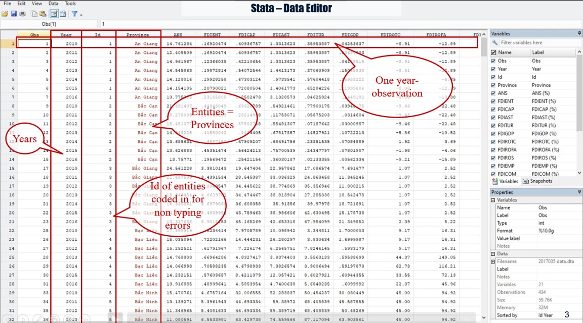
In this sample, “id” represents the entities as Vietnam provinces that we code them in number; and “year” represents the time variable (t). Note that you should make attention for assuring that all data of one thing such as one entity are coded exactly the same. If not, Stata will count as another thing or ignore it.
The objective of our research aims to study the relationship between foreign direct investment (FDI) and sustainability at provincial level in a developing host country as Vietnam for the period between the years of 2010 and 2016.
Here are the variables of our research; in which Dependent variable is the adjusted net savings that assess the sustainable development of Vietnam provinces. In total, we have 11 independent variables that are distinguished in three groups, including: 3 variables associated with the FDI inflow stocks; 5 variables associated with the employment in FDI sector, and 3 variables associated with the performance of FDI in provinces. And, 2 control variables are size and economic growth of province.

Practical regression process
Now, we apply the process of selecting the regression model for panel data (between Pooled OLS Model, Random-Effects Model and Fixed-Effects Model) of Dougherty (2011) for our panel data of Vietnam provinces in period from 2010 to 2016.

Source: Dougherty (2011, p.421)
For the first step, our sample can be considered as random sample because of our choice in time-span and FDI sector at provincial level in Vietnam.
So, we go into the second step of the Process of choosing regression model for panel data, in which we perform both fixed effects and random effects regressions by using Stata.
The Stata command to run fixed/random effects is xtreg.
Before using xtreg you need to set Stata to handle panel data by using the command xtset. Type: xtset Id Year, yearly. Note that Stata distinguishes capital letters, so you must type exactly the variable name. Or you can click this command on the Stata’s Menu by avoiding typing errors.
In this case, “Id” represents the entities that is Vietnam provinces; and “Year” represents the time variable t.
As the panel data has been handled, we can now run the fixed-effects model by using the Stata command xtreg with dependent variable ANS and 13 variables, including 11 independent ones and 2 control variables in our panel data.
Type: xtreg ANS FDIENT FDICAP FDIAST FDIEMP FDICOM FDIWAG FDITUR FDIGDP FDIROTC FDIROFA FDIROS Size GDPgrowth, fe.
Or you can click this command on the Stata’s Menu by avoiding typing errors. Note that the option fe should be chosen for the fixed-effects model.

To compare the results with random-effects model that will be performed later; we must now store the results with fixed-effects regression by using the command “estimates store fixed”.
Then, we run the random-effects model by using the Stata command xtreg with the same variables by choosing the option re
Type: xtreg ANS FDIENT FDICAP FDIAST FDIEMP FDICOM FDIWAG FDITUR FDIGDP FDIROTC FDIROFA FDIROS Size GDPgrowth, re.
Or you can click this command on the Stata’s Menu by avoiding typing errors.

Also, we save the estimates by using the command “estimates store random”.
For comparing fixed and random-effects models, we perform now the Hausman test by typing” hausman fixed random
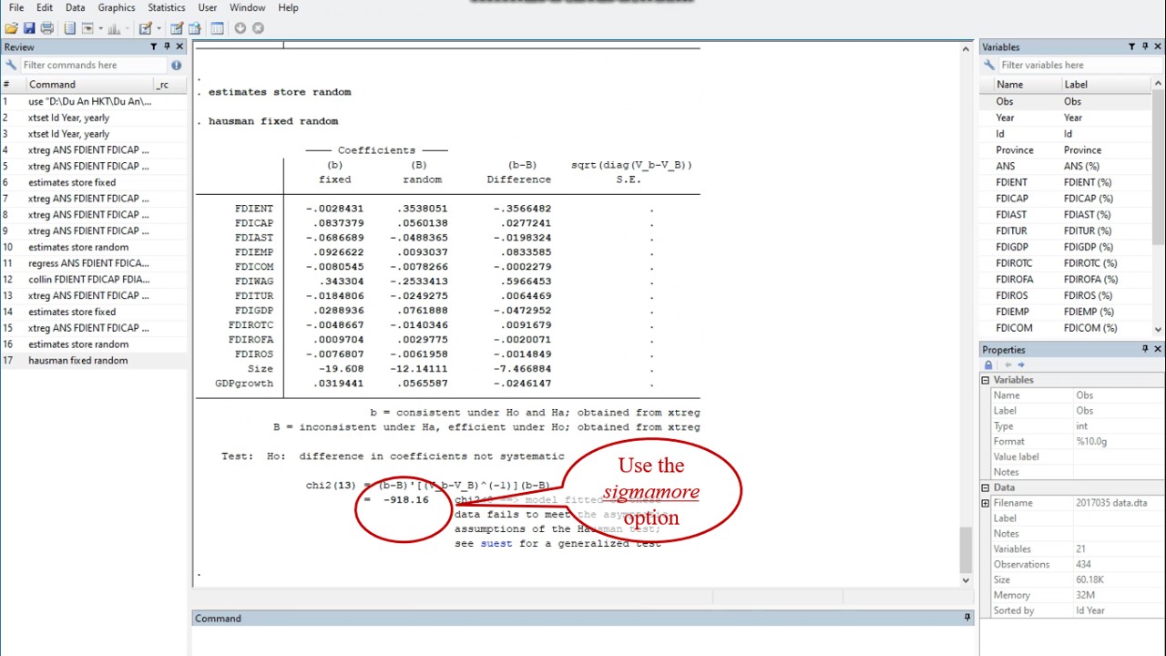
The negative sign can arise if different estimates of the error variance are used in forming variance of b and variance of capital B. In that case, we need to use the sigmamore option, which specifies that both covariance matrices are based on the (same) estimated disturbance variance from the efficient estimator.
Type: hausman fixed random, sigmamore

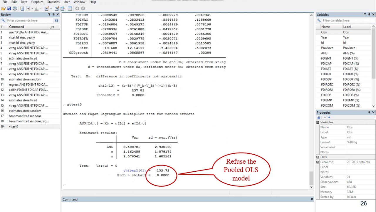
By focusing on the DWH test, we determine whether there are significant differences in the coefficients. This significant Hausman test allow us to accept the null hypothesis by indicating that the Fixed-effects model is appropriate.
By caution, it is necessary to test the presence of random effects by using Breusch-Pagan Lagrange multiplier. We can see that the result of this test is significant by indicating random effects and refusing the Pooled OLS model.
As the Hausman test has eliminated the random-effects model; and Lagrange multiplier has refused the Pooled OLS model. We select with confidence now Fixed-effects one.
We must check the Heteroskedasticity test for the selected Fixed-effects model by using the command xttest3. This is a user-written program, to install it type: ssc install xtest3
Because, Stata stored recently the results of random-effects model; we rerun the fixed-effects regression; then run Heteroskedasticity test. The null is homoskedasticity.

And our significant test rejects the null and indicates that our Fixed-effects model has a heteroskedasticity problem.
Hence, we use the option robust to correct for this regression model by typing the xtreg with 2 options such as robust and fe.

Finally, the robust Fixed-effects model is used for assessing the proposed research hypotheses in our research.

Please see the detail results and analysis in our article Nguyen Hoang Viet, Phan Thanh Tu and Lobo Antonio (2019)
Other tests / diagnostics
Testing for time-fixed effects
To see if time fixed effects are needed when running a FE model use the command testparm. It is a joint test to see if the dummies for all years are equal to 0, if they are then no time fixed effects are needed (type help testparm for more details).
After running the fixed effect model, type: testparm i.year
NOTE: If using Stata 10 or older type:
xi: xtreg y x1 i.year, fe
testparm _Iyear*

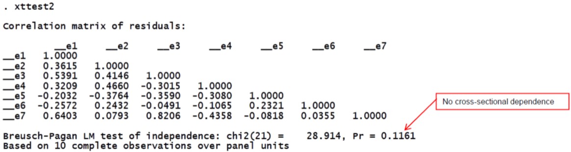
Testing for cross-sectional dependence/contemporaneous correlation: using Breusch-Pagan LM test of independence
According to Baltagi, cross-sectional dependence is a problem in macro panels with long time series (over 20-30 years). This is not much of a problem in micro panels (few years and large number of cases).
The null hypothesis in the B-P/LM test of independence is that residuals across entities are not correlated. The command to run this test is xttest2 (run it after xtreg, fe):
xtreg y x1, fe
xttest2
Type xttest2 for more info. If not available try installing it by typing ssc install xttest2
Testing for cross-sectional dependence/contemporaneous correlation: Using Pasaran CD test
As mentioned in the previous slide, cross-sectional dependence is more of an issue in macro panels with long time series (over 20-30 years) than in micro panels.
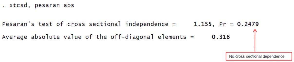
Pasaran CD (cross-sectional dependence) test is used to test whether the residuals are correlated across entities*. Cross-sectional dependence can lead to bias in tests results (also called contemporaneous correlation). The null hypothesis is that residuals are not correlated.
The command for the test is xtcsd, you have to install it typing ssc install xtcsd
xtreg y x1, fe
xtcsd, pesaran abs
Had cross-sectional dependence be present Hoechle suggests to use Driscoll and Kraay standard errors using the command xtscc (install it by typing ssc install xtscc). Type help xtscc for more details.
Testing for heteroskedasticity
A test for heteroskedasticiy is avalable for the fixed- effects model using the command xttest3.
This is a user-written program, to install it type:
ssc install xtest3
xttest3
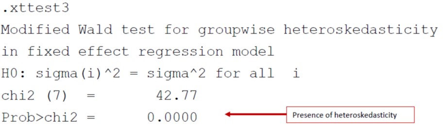
The null is homoskedasticity (or constant variance). Above we reject the null and conclude heteroskedasticity. Type help xttest3 for more details.
NOTE: Use the option ‘robust’ to obtain heteroskedasticity-robust standard errors (also known as Huber/White or sandwich estimators).
Testing for serial correlation
Serial correlation tests apply to macro panels with long time series (over 20-30 years). Not a problem in micro panels (with very few years). Serial correlation causes the standard errors of the coefficients to be smaller than they actually are and higher R-squared.
A Lagram-Multiplier test for serial correlation is available using the command xtserial.
This is a user-written program, to install it type ssc install xtserial
xtserial y x1
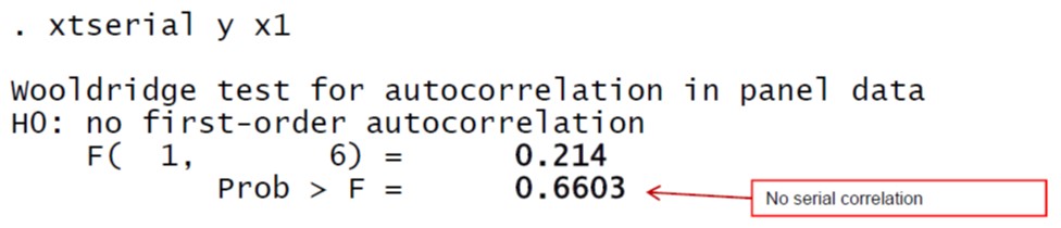
The null is no serial correlation. Above we fail to reject the null and conclude the data does not have first-order autocorrelation. Type help xtserial for more details.
Testing for unit roots/stationarity
Stata 11 has a series of unit root tests using the command xtunitroot, it included the following series of tests (type help xtunitroot for more info on how to run the tests):
“xtunitroot performs a variety of tests for unit roots (or stationarity) in panel datasets. The Levin-Lin-Chu (2002), Harris-Tzavalis (1999), Breitung (2000; Breitung and Das 2005), Im-Pesaran-Shin (2003), and Fisher-type (Choi 2001) tests have as the null hypothesis that all the panels contain a unit root. The Hadri (2000) Lagrange multiplier (LM) test has as the null hypothesis that all the panels are (trend) stationary.
The top of the output for each test makes explicit the null and alternative hypotheses. Options allow you to include panel-specific means (fixed effects) and time trends in the model of the data-generating process” [Source: type help xtunitroot]
If Stata does not have this command but can run user-written programs to run the same tests. You will have to find them and install them in your Stata program (remember, these are only for Stata 9.2/10). To find the add-ons type:
findit panel unit root test
A window will pop-up, find the desired test, click on the blue link, then click where it says “(click here to install)”
For more info, please see Torres-Reyna (2007).
Good post but I was wondering if you could write a litte more on this topic? I’d be very grateful if you could elaborate a little bit further. Thanks!
Somebody essentially assist to make critically posts I would state. This is the first time I frequented your web page and so far? I surprised with the research you made to make this actual publish extraordinary. Fantastic job!
I was very pleased to find this web-site.I wanted to thanks for your time for this wonderful read!! I definitely enjoying every little bit of it and I have you bookmarked to check out new stuff you blog post.