Different regression models with Panel data (fixed-effects, random-effects, and pooled OLS)

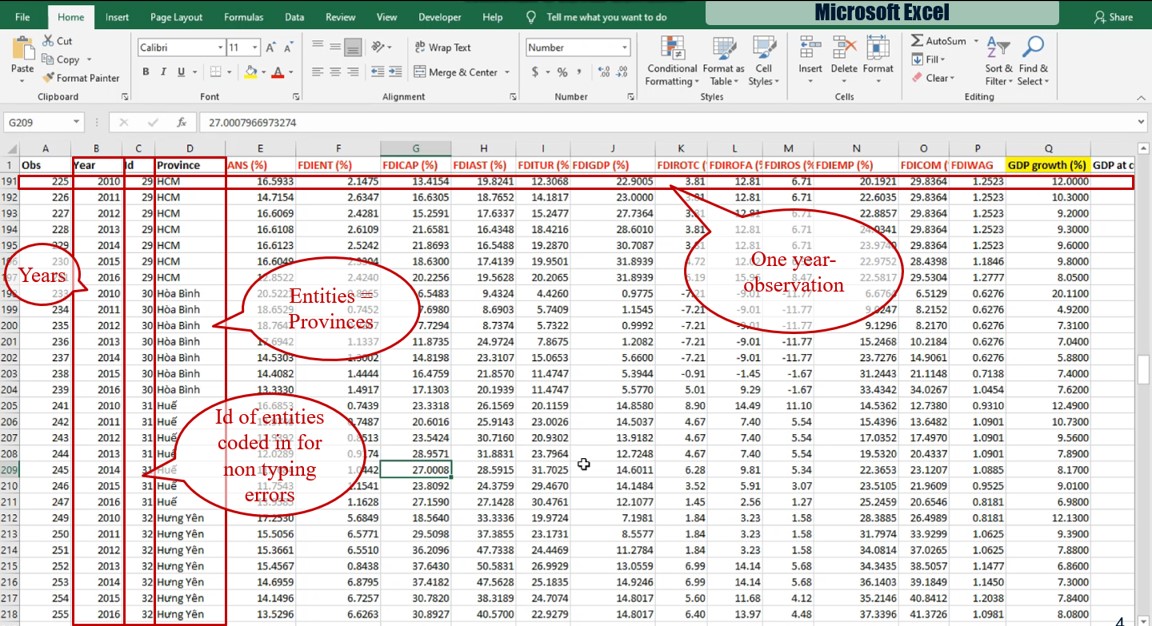
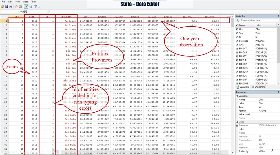
Panel data, also known as longitudinal or cross-sectional time-series data, is a dataset in which the behaviors of entities are observed across time. These entities could be states, companies, individuals, countries etc. Panel data allows us to control for variables we cannot observe or measure across entities; or variables that change over time but not across entities

Panel data allows you to control for variables you cannot observe or measure like cultural factors or difference in business practices across companies; or variables that change over time but not across entities (i.e. national policies, federal regulations, international agreements, etc.). This is, it accounts for individual heterogeneity.

With panel data you can include variables at different levels of analysis (i.e. students, schools, districts, states) suitable for multilevel or hierarchical modeling. Some drawbacks are data collection issues (i.e. sampling design, coverage), non-response in the case of micro panels or cross-country dependency in the case of macro panels (i.e. correlation between countries).

In this document we focus on techniques use to analyze panel data, including:

Fixed-effects model

We use fixed-effects model whenever we are only interested in analyzing the impact of variables that vary over time. This model is “designed to study the causes of changes within an entity. A time-invariant characteristic cannot cause such a change, because it is constant for each entity” (Kohler and Kreuter. 2008).

Fixed-effects model explores the relationship between independent variable and dependent variable within an entity as province in our empirical study. Each entity has its own individual characteristics as independent variables, that may or may not influence the dependent variable.

When using Fixed-effects model, we assume that something within the individual may impact or bias the independent variables and we need to control for this. This is the rationale behind the assumption of the correlation between entity’s error term and independent variables. Fixed-effects model remove the effect of those time-invariant characteristics so we can assess the net effect of the independent variables on the dependent one.

Another important assumption of the Fixed-effects model is that those time-invariant characteristics are unique to the individual and should not be correlated with other individual characteristics. Each entity is different therefore the entity’s error term and the constant (which captures individual characteristics) should not be correlated with the others. If the error terms are correlated, then Fixed-effects model is no suitable since inferences may not be correct, and we need to consider the random-effects model, this is the main rationale for the Hausman test.

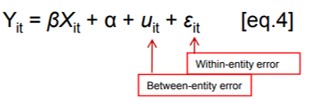
The equation for the fixed effects model becomes:

Y_it = α_i + β_iX_it + u_it

Where:

• αi (i=1….n) is the unknown intercept for each entity (n entity-specific intercepts).
• Yit is the dependent variable (DV) where i = entity and t = time.
• Xit represents one independent variable (IV),
• β1 is the coefficient for that IV,
• uit is the error term

“The key insight is that if the unobserved variable does not change over time, then any changes in the dependent variable must be due to influences other than these fixed characteristics.” (Stock and Watson, 2003, p.289-290). “In the case of time-series cross-sectional data the interpretation of the beta coefficients would be “…for a given country, as X varies across time by one unit, Y increases or decreases by β units” (Bartels, Brandom, “Beyond “Fixed Versus Random Effects”: A framework for improving substantive and statistical analysis of panel, time-series cross-sectional, and multilevel data”, Stony Brook University, working paper, 2008). Fixed-effects will not work well with data for which within-cluster variation is minimal or for slow changing variables over time.

Another way to see the fixed effects model is by using binary variables. So the equation for the fixed effects model becomes:

You could add time effects to the entity effects model to have a time and entity fixed effects regression model:

Control for time effects whenever unexpected variation or special events my affect the outcome variable.

A note on fixed-effects that: “…The fixed-effects model controls for all time-invariant differences between the individuals, so the estimated
coefficients of the fixed-effects models cannot be biased because of omitted time-invariant characteristics…[like culture, religion, gender, race, etc]. One side effect of the features of fixed-effects models is that they cannot be used to investigate time-invariant causes of the dependent variables. Technically, time-invariant characteristics of the individuals are perfectly collinear with the person [or entity] dummies. Substantively, fixed-effects models are designed to study the causes of changes within a person [or entity]. A time-invariant characteristic cannot cause such a change, because it is constant for each person.” (Kohler, Ulrich, Frauke Kreuter, Data Analysis Using Stata, 2nd ed., p.245).

Random-effects model

The rationale behind random effects model is that: unlike the fixed-effects model, the variation across entities is assumed to be random and uncorrelated with the independent variables included in the model. So, “…the crucial distinction between fixed and random effects is whether the unobserved individual effect embodies elements that are correlated with the regressors in the model, not whether these effects are stochastic or not” (Green, 2008, p.183).

Random effects assume that the entity’s error term is not correlated with the independent variables which allow for time-invariant variables to play a role as independent variables.

If we have reason to believe that differences across entities have some influence on our dependent variable, then we should use random effects. An advantage of random effects is that: we can include time invariant variables (such as superficies of province). In the fixed effects model, these variables are absorbed by the intercept.

The random effects model is:

Random effects assume that the entity’s error term is not correlated with the predictors which allows for time-invariant variables to play a role as explanatory variables.

In random-effects, we need to specify those individual characteristics that may or may not influence the independent variables. The problem with this is that some variables may not be available therefore leading to omitted variable bias in the model.

RE allows to generalize the inferences beyond the sample used in the model.

Pooled OLS model

Pooled data occur when we have a “time series of cross sections,” but the observations in each cross section do not necessarily refer to the same unit. In panel data, Pooled OLS (ordinary least squares) can be used to derive unbiased and consistent estimates of parameters even when time constant attributes are present, but random effects model will be more efficient.

Fixed effects model is a feasible generalized least squares technique which is asymptotically more efficient than Pooled OLS when time constant attributes are present. Random effects model adjusts for the serial correlation which is induced by unobserved time constant attributes.

The Pooled OLS model is:

Y = α + β_iX_i + ε

Choosing the right model

The process of selecting the regression model for panel data (between Pooled OLS Model, Random-Effects Model and Fixed-Effects Model) is discussed in research of Dougherty (2011) as depicted in following Figure.

Source: Dougherty (2011, p.421)

Specifically, the process begins with considering whether the observations are a random sample from a given population, that is a subset of individuals randomly selected by researchers to represent an entire group as a whole. In the first step, we determine if these observations are a random sample, if this is the case, we perform the next step, otherwise we use fixed-effects model as the final decision.

In case of random sample, we continue the second step by performing both fixed-effects and random-effects models, then we compare these models by using the Hausman test, also known as the Durbin-Wu-Hausman or DWH test, where the null hypothesis is that the preferred model is random effects versus the alternative the fixed effects (see Green, 2008, chapter 9). It basically tests whether the unique errors (ui) are correlated with the regressors, the null hypothesis is they are not.

So, If the Hausman test indicates significant differences in the coefficients; final choice consists in Using fixed-effects model.

In contrast for the third step, the Lagrange multiplier is used to decide if the random-effect model or the pool OLS model is suitable for the research. The null hypothesis in the LM test is that variances across entities is zero. This is no significant difference across units. Specifically, if LM test indicate the presence of random effects; random-effects model will be chosen; otherwise pooled OLS model will be our final decision.